27 Forecasting and Problem Spotting
Taeke
de Jong, Hugo Priemus
27.1 Problem spotting..................................................... 1
27.2 Systems’ consideration.......................................... 2
27.3 Criteria of assessment........................................... 2
27.4 Establishing alternatives........................................ 3
27.5 Evoking system behaviour..................................... 4
27.6 Generalisations...................................................... 4
27.7 Curve fitting............................................................ 5
27.8 Causal pre-suppositions........................................ 6
27.9 Constraints............................................................. 6
27.10 Sensitivity............................................................... 7
27.11 Parameters............................................................. 8
27.12 External factors..................................................... 8
27.13 Scenarios............................................................... 9
27.14 Sector scenarios................................................... 9
27.15 Policy balancing................................................... 11
27.16 Scenario development......................................... 11
27.17 Limitation shows the master................................ 12
Scientific forecasting and problem spotting calls for models of a reality within which one tries to make predictions. In this Chapter some crucial concepts will be treated that are involved during modelling. They are treated in large-scale examples, since examples like these feature fewer boundary conditions complicating forecasting than examples on a small scale.
Forecasting
the size of the world's population is after all, easier than the one of an
individual household. As long as one believes in the human freedom of choice, forecasting on the level of the individual is
even impossible. Only with large numbers may a
meaningful relation be established, up to now, of one event A with the possible
results W (chance = A/W, see page ).
That is the reason why ‘chance’ is a central model in a science aiming at generalising statements for the future. These are needed to come to grips with the future and its problems.
Forecasting study cannot do without this concept of chance. At
increasing numbers, the choices of individuals group themselves around an
increasing stable, 'reliable', mean against which the deviation of individual cases may be measured. From a
range reliable numbers or averages as a function of time, a trend can be read, that may be generalised
eventually to a mathematical formula (curve
fitting).
If this trend is undesirable, we have spotted a problem. A sequence of numbers X may be related to any other sequence of numbers Y -not only to a time axis- if in the swarm of graphical dots a line can be drawn, the line of regression.
Such a line of regression can be arrived at by many different (non-declarative) mathematical formulae.
In forecasting study relations of this type are important in order to arrive at statements like 'If x then y'. That does not say yet that x causes y. However, the effort to explain a statistical coherence remains important.
Departing from such a causal explanation one can sometimes arrive at a mathematical formula. Only who can explain, can predict with authority?[1]
27.1 Problem spotting
The set of all problems is a set of probable, but not desirable futures. An applied empirical study starts with formulating such an undesirable probability (problem statement or formulation). A problem is probable and so can be forecast (signalled). Problem signalling already pre-supposes two predictions: the prediction of wishes and of probabilities. So the problem statement is not the real beginning, but part of an empirical cycle[2], in which problem statement, forecast, new problem statement produce one another
|
|
|
Figure 1 Futures and their modalities |
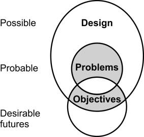
The aim, or objective (several aims), of the study points from that problem to the more desirable future. The future aimed at, from which the aim of the study has been derived, is per definition desirable and not probable (one does not aim at realising tomorrow’s sunrise) but possible; as far as we can see. Since an aim is not probable, it can not be forecast. So it must be chosen, posed, often even designed. An aim is an abstract pre-design of an alternative deemed possible for the present situation and its probable development (zero variant). These abstract concepts refer for everyone to comparable situations that usually remain implicit in order ‘not to exchange aim and means’, regardless of the level of abstractness, such as increased safety or accessibility. However, what is termed ‘aim’ and ‘means’ depends on the level of abstraction. The acquisition of a government subsidy can be an aim for a community, but for the country it is a means for a higher aim.
27.2 Systems’ consideration
From the problem formulation, further demarcations may be derived allowing separation of a dynamically variable and researchable system from a context that is largely independent (systems analysis)[3].
This also results in the constraints within which the system must function. In addition, the problem formulation generates clues how system and context should be reduced to a composite of researchable, valid and reliable (see page ) variables (operationalisation) with the mutual relations (modelling in functions). The functions are going to be mutually related, so that the output of one function becomes the input of one or more subsequent functions (systems modelling).
An inter-action with a causality in two directions often occurs. These relations within and between functions pre-suppose previous empirical study (empirical cycle) that demonstrated such a relation or that seems probable by reflection.
Within the demarcation, the constraints and from the objective, the alternatives are designed (means, pre-supposed solutions, encroachments, with the rôle of hypotheses[4] that can be checked). These alternatives must be weighed (assessment). Against which values or criteria? Between vague values and precise criteria, a wide range of gradation exists.
27.3 Criteria of assessment
It is impossible to imagine criteria and norms without objectives underlying them and objectives without the basis of individual or social values. On the other hand, it is possible to imagine values that have not been worked out into objectives as yet and objectives not yet associated with norms. These concepts operationalise subsequently increasingly concretely a desirable future, so far as is possible, so that it may be tested. Along these lines public safety is an important social value that may be made workable (operational) in more specific objectives, like better lighted public spaces, worked out into norms for lighting that can be controlled. The English language is rich in terms for objectives in the various stages between what is strategic and what is operational. In the following diagram they have been put in a conditional sequence.
|
|
|
Figure 2 From possibility to norm |
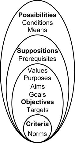
However, one is well advised to remember that values have been founded on a body of implicit conditions, pre-suppositions and imaginations: culture. As far as they are related to truth, these are the conditions from classical logic (if…then, if…if, then and only if, see page ). They yield a consistency check with regard to the logic of the discourse, not yet with regard to causal correctness of the premises in the wider area of probabilities. An example: “If public illumination ameliorates security, then illumination will make this insecure, not illuminated place more secure.” However, the premise that illumination ameliorates security is always a context-sensitive causal pre-supposition. Moreover, in each and every objective also technical conditions are hidden, allowing checking. They are often implicit (lamps exist, the electricity needed is available and affordable, the neighbours do not experience illumination as cumbersome, implementation is feasible in the municipal council). They delimit what is possible and feasible from what is impossible and are creating room for what is improbable (conditions)[5].
All these conditions, values and their development into objectives and criteria, should be part of the problem formulation. But, then the problem formulation would encompass the study as a whole; it is more advisable to make a rough sketch first to be added to and updated during the study, in periodical consultation with the initiator.
The central objective of this is a reduction in which underlying values, conditions, suppositions, means, conditions and possibilities of the problem investigation have been omitted.
However,
the investigator is obliged to identify as many of the prevailing values as
possible and to make them explicit in order
to operationalise them in
criteria for the assessment of alternatives. In
the classical scheme of Findeisen and Quade (see page ), this part of the systems' analytical
study is rendered with: 'Identifying, designing and screening the
alternatives'.
27.4 Establishing alternatives
One line of text might make a hypothesis, but not a full-fledged design. The systems’ analysis requires different hypotheses (alternatives) to test the completeness of the system. Alternatives may emerge for which the system has not an answer yet.
The classical model of the empirical cycle lacks an instruction for establishing hypotheses. The establishing of hypotheses is 'free'. Scientifically spoken, anything can be argued or drawn up, until the hypothesis is refuted[6] or replaced by a better alternative.
But, if the hypothesis is an architectural design, establishing the hypothesis is an important part of the study by design, highlighted in other Chapters of this book. In the process of building generating an alternative for the present situation (zero-variant) may entail 95% of the studying effort. Often just one alternative exists, to be varied upon at best during the process. There is then less time available for problem analysis. In architectural design many more (detailed) decisions are taken than for which the objective can be directive; often even a tacitly pre-supposed type of building or neighbourhood.
The decisions as to shape and
structure outside of the objective - usually regarded as of secondary
importance - require insight into a combinatorial explosion of possibilities
(see page ).
In order to reduce them, the designer uses not only the problem formulation and the objective (the site and the programme of requirements), but also existing examples (precedents, design study) and types (typological study). The designer is guided by a global concept that allows more aims than formulated in words by the initiator. A sustainable building must be able to serve in a different context after selling it subsequent owners ('robustness' of the design).
If
the designer varies the context taken to be obvious in the problem analysis as
well (study by design[7]), the design may lead to a
review of the perception of the problem; and, by the same token, of the systems
analysis. This feed-back arrow is missing in
the schema of Findeisen et al. on page .
27.5 Evoking system behaviour
Calculating the consequences of an action, alternative, design or hypothesis (evaluating study ex ante, see page ) requires prediction. Each prediction pre-supposes a context, within which the proposed action functions. Change in context (perspective) changes the consequences of the action.
The sensitivity of the prediction for these changes cannot be avoided in applied study by pre-supposing 'other things being equal' (ceteris paribus). One has to highlight the consequences of several actions in several perspectives in order to achieve a more general insight into 'system behaviour' under different circumstances and actions. The construction of these perspectives (future contexts) with unexpected aspects and decision moments (scenarios) will be dealt with in a following paragraph.
Scenarios play a rôle within the predictions in the system itself as providers of external exogenous variables (parameters) in the equations on which the systems' model has been built. By changing these parameters in the equations per scenario, additional consequences may emerge.
27.6 Generalisations
The possibility of forecasting and prediction depends on external generalisations from previous experiences (empiry). Not only external ones apply, also internal. Particularly the use of the average as the most important form of statistical generalisation and its extrapolation in time, meets with opposition from scientific disciplines supposed to deal with a large variety in objects and contexts: especially ecology, organisational science[8] and designing. In ecology this reduction to an average by the analysis of ecosystems is known as the 'mean-field assumption' (see following diagram).
|
|
|
|
|
|


This
reduction can smooth local variations in such
a way, that the character of the
object and its context evaporate. At the same time the survey of the specific
possibilities of the site ceases to exist. The statistical measure for deviation cannot replace this variation.
In evolutionary ecology[10] especially a few cases of exception, outside of the 95% area, determine the future course of the ecological process, since these rarities may lead in particular to the emergence of new species and systems. This suggests mathematical chaos functions, featuring, by means of iteration an unpredictable course; they are very sensitive to the minutest variations at first input. Rounding-off strategies in different computer brands may even lead to the circumstance that one and the same formula yields a different outcome on two distinct machines.
All this does not derive from the fact that forecasts, or less explicit, expectations, are the base of acting. By way of an example, we select the growth function of a population.
27.7 Curve fitting
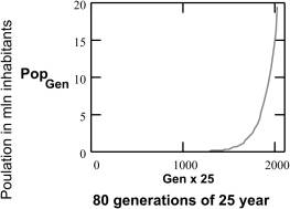
The population of the Netherlands has grown during the last three centuries as follows.
|
|
|
Figure 4 Actual growth of the population in the Netherlands |
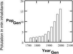
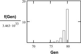
The bars in this graph comprise class intervals of 25 years (interpreted here as generations) with the population figures levelled out over the period. First of all, the progress recalls an exponential function f(x) = exp(x); after the industrial revolution reaching the country around 1800.
In the figure below a part of this function from the beginning of the Christian era has been drawn for the last 10 generations (1750 – 2000 AD). For x Gen (generations) has been substituted.
|
|
|
Figure 5
f(Gen)=exp(Gen) |
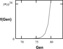
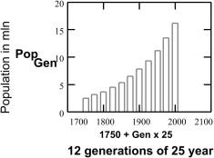
This function leads from 0 persons in year 0, to an unlikely high population figure of f (80)= 5.541 x 1034 in the year 2000 (generation 80). If we divide this number by the current population size of 16 million Dutch (wo)men f (80)/ 16 = 3.463 x 1033, the first parameter materialises in the model that as denominator reduces the last generations (80) to 16 million.
|
|
|
Figure 6 The same with parameter |
This does not reflect reality well. The mathematical representation of population growth is differing too much from actual data.
27.8 Causal pre-suppositions
Each generation comprises the number of parents, times their average number of children, plus the parents themselves. In each following generation children become parents, and parents grandparents. They die; and the grandparents should be subtracted from the following generation. This can be rendered in an iterating formula[11].
PopGen+1 : = Children x PopGen
+ ParentsPopGen – GrandparentsPopGen - 1
|
|
|
Figure 7 The exponential growth of a population |
For this graph we had to fix the first generation to two people in the year 0 and the number of children to a parental couple through all these centuries to 1.034 on average.
This formula cannot be extrapolated readily to earlier years. However, the slice since 1750 starts to resemble reality. A function allowing more extrapolation would require for the aim of this discourse too many additional parameters from earlier contexts (for instance: a parameter working out negatively for the emergence of epidemics of plague at certain population densities and a medieval state-of-the-art of medical science).
|
|
|
Figure 8 Slice of Figure 7 |
27.9 Constraints
If a population approximates its limits, growth lessens. For such a phenomenon mathematics offers the logistical curve.
|
|
|
Figure 9 The logistical curve |
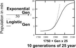
In a non-iterative form, the formula
for exponential growth has an exponent, compare page ; the logistical curve is an
extension with two parameters, the first of which initiates the restriction.
ExponentialGen = Pop 0 x ChildrenGen
LogisticalGen = Pop 0 x ChildrenGen x restriction / (ChildrenGen+ Childrena)
The second parameter, exponent ‘a’ in the denominator of the logistical function, regulates the speed of growth.
27.10 Sensitivity
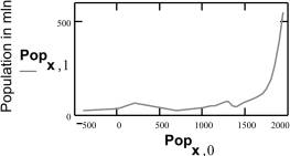
The iterating functions leading to fractal geometry and chaos theory have proven that systems may vary vastly by minimal differences in input and parameters (sensitivity)[12]. The following function (chaos function) resembles at the value a = 2 of parameter a the logistical curve.
|
|
|
Figure 10 xGen-1
= axGen - axGen2 ChaosGen = 30xGen + 2 a = 2 |
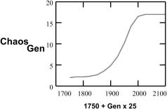
For an initial value X0 = 0.0016 this function is congruent with the growth of the Dutch population. In order to match it, one must multiply by 30 and to get it to the right height one should add 2. Then, it 'forecasts' a stability following the year 2000.
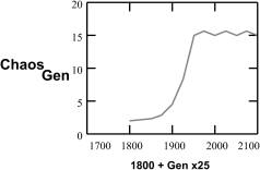
However, if one chooses for parameter a = 3, the function starts to flutter.
|
|
|
Figure 11 a = 3 |
At a = 4 the function becomes chaotic.
|
|
|
Figure 12 a = 4 |
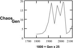
And at a = 4.1, an entirely different graph results.
27.11 Parameters
A quiet constraint like lack of space results in a quiet smoothing, while wars and epidemics result in wild fluctuations. Rather more causally, fluctuations like that are simulated by the Lotka-Volterra function for preys (like people) and their predators (for instance the plague bacteria or other people in their guise of enemy).
|
|
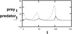
In the case of this function time is input (here at a scale implying nothing particularly from 1 to 150), with the densities of prey and predator for output. They are inter-changing as ‘causation’ of rising and declining. For the densities initial amounts should be stated; as well as the value of the four parameters.
These regulate the waxing of prey if there are no predators, the percentage of animals of prey caught, the death and emigration of predators and increase by consumption of prey. If the value of parameters of this type cannot be ascertained by empirical research, it is possible to arrive at a state that proves to match time series of the past (calibration). In both cases it imports to check the sensitivity of the model to parametrical selection and to report on it. Varying parameters as to their effect on the graph is no punishment anymore, considering current computer capability, and sometimes provides outright sensations. But the larger the number of parameters one may use as 'buttons on the piece of equipment', the more difficult it becomes to determine the influence of each button separately on the result. The influence of one parameter can change drastically, if one turns other dials.
If one has 6 buttons at one's disposal, each with at least 10 positions, like in the Lotka-Volterra function, the minimal number of combinations, 610, is already not to be surveyed. Which of the resulting 610 functions should one choose for the model desired?
With the explosion in terms of
number of combinations (see page ) of the tuning of parameters the
fringes of realistic modelling are attained often in sciences markedly
sensitive to context; as there are architecture, ecology and organisational
science.
27.12 External factors
In the case of the Lotka-Volterra function the predator, initially regarded as external factor, has been assimilated within the model (internalisation).
While the predator was directly dependent on the availability of prey, they formed together a ‘system’ that might be modelled with inter-changing causality. Obviously, internalisation cannot digest everything. Quite a few external influences just have to be stated, or to be varied for some scenarios.
The presumable course of Europe's population[14] shows the consequences of a lot of unidentified external factors, although it is known, that the plague, The Black Death, raged at the end of the Middle Ages.
It seems as if an internal drive to exponential growth is always stinted, until all brakes vanish in modern times. Which factors have been responsible for that: spatial, ecological, technical, economical, cultural, managerial? Pre-suppositions concerning size and nature of immigration and emigration are crucially important for real-life population prognoses.
|
|
|
Figure 14 Population development in Europe |
Determining the parameters for fluctuations like these, and establishing the functions by which they operate, requires more data and more detailed analyses. They may result in data files of parameters that may be consulted through the systems' model during calculation with 'if.. then..' statements.
They require knowledge of the influence of spatial, ecological, technical, economical and managerial developments in time series[15].
Among all influences in the case of population forecasts, for instance, the crucial factor of the average number of children per household (fertility) determines the factor of reproduction. The shorter the time-span of validity of the forecasting, the longer the time series on which the forecast is based (founding period); and the more substantial the explanation enabled by the independent variables, the more reliable the forecast. The Statistics Netherlands (CBS) publishes a population prognosis on an annual basis (in Monthly Statistics for the Population).
27.13 Scenarios
Although scenarios are made for many reasons (insight, strategy, management inside and inter-action between organisations) they are considered here as purveyors of exogenous variables in order to serve systematically forecasting and problem spotting study.
A scenario is not a calculated (prognosis) or an assumed probable future (perspective). A scenario is a time series projected into the future within which managerial, cultural, economical, technical and spatial influences (stemming from actors in these different sectors) are varied consistently and plausibly. It is the description of a possible future, partly designed, that corresponds partly to prognoses and perspectives and that may contain partly policy decisions.
|
|
|
Figure 15 Possible, probable, desirable, image of future and scenario |
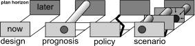
In
this figure, rendered in a sequence lacking
intention, it is represented that the design
tries to project one whole image on the planning horizon, while the prognosis delimits there an area that might be
put to work in a scholarly way. In this area in which the subsequent consequences
are depicted, there just might be another area than where preceding causes are
dwelling. The prognosis departing from a plan,
not from the current situation (evaluation ex ante, effect
analysis, see page ), is taking its bearings on uncertain
pre-suppositions regarding context (boundary conditions; the tiny arrows in the
last drawing).
Policy punctuates a path with limiting values when a part of the policy goal should have been reached (target figure). In principle, a scenario compromises all components although one component may take the lead. If the starting point is the design with a final stage and from there the reasoning is backwards (back-casting), one talk about a prospective scenario, in other cases of a projective scenario. If prognosis stands central, the parlance is 'trend-scenario'; and if, on the contrary, unexpected events play a more important rôle, ‘surprise-scenario’.
If policy objectives pre-dominate, normative- scenario is the word.
In the policy time-path decision moments may materialise that can give the scenario a twist. In order to survey consequences of such decisions, policy scenarios or exploring scenarios are made, with alternative scenarios branching out tree-wise.
27.14 Sector scenarios
Scenarios exist emphasising particularly political, cultural, economical, technical, ecological (demographical) or spatial sectors for a driving force. Their yardsticks, research methods and variables differ greatly, which makes them difficult to combine and integrate. Sector scenarios like that are made, for instance, by the Netherlands Bureau for Economic Policy Analysis (CPB, economical scenarios), the Social and Cultural Planning Bureau (SCP, cultural scenarios), the Rijksinstituut voor Volksgezondheid en Milieu (RIVM, ecological and nature scenarios) and the AVV (mobility scenarios).
Often, they are cross-wise combined to more integral scenarios, contrasting with one another (extreme scenarios or contrast scenarios). This contrast is called for to make effective sensitivity analyses in systematic study of the future.
|
|
|
Figure 16 Cross-wise integration of sector scenarios |
With the 6 sectors mentioned previously, 15 quartets of this type can be produced.[16]
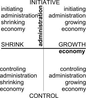
One may also contrast, for instance, policy (steering <> following) with culture (tradition orientated <> experiment orientated), technique (combining <> specialising), ecology (homogeneous <> heterogeneous) or space (deconcentration <> concentration).
CPB scenarios vary with the relative strength of European economy in the competition with American or South-East Asiatic clusters, or with the effectiveness of co-operation within Europe itself: Global Competition, Divided Europe and European Co-ordination.
However, these sectors have different time horizons and dynamics; this hinders contrasting them mutually. The figure below illustrates this as a series of trend-scenarios fluctuating between the extremes.
|
|
|
Figure 17 Difference in dynamics between trends |
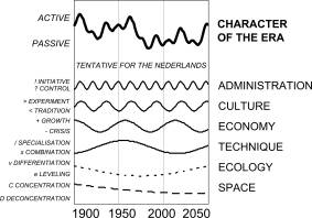
In this figure the face of the time is an addition of rather dubious sector trends, depending on the notion that each action calls for an anti-thetical (Hegelian) reaction; so that, between two extremes, an oscillating movement emerges; here depicted as a clean sinus curve. Now imagine that these sinuses have been calibrated on the century now passed; while it has been shown that policy fluctuates by seven years between guiding and following, and culture is shifting within 14 years between traditional and experimental orientation; and so forth
What name should be given to the extremes of their super-position? 'Active' and 'passive' are the, scarcely meaningful, terms chosen here. Balancing developments in different sectors is usually left to politics. Nevertheless, it establishes a scientific challenge that gets attention especially in ecological policy: how does one weigh environmental interest against economical and spatial priorities?
27.15 Policy balancing
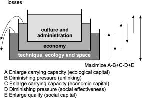
Between the sectors one can pre-suppose conditionality. Technique has its ecological conditions: without food, water or materials, technique would not exist. There are technical conditions for the economy: without dikes in our low delta lands, the economy would not exist either, etc. This leads to a model of sustaining capacity. In it, the sectors do not pre-suppose one another causally (a certain technique leads to a certain economy), but conditionally (a certain technique makes different economies possible).
|
|
|
Figure 18 Balancing between sectors |
One may also try to make a more technical judgment, for instance between nature areas and airports. The product of their scarcity in a wide surroundings and the viability to generate them within a particular time, provides a yardstick for comparison.
|
|
|
Figure 19 Technical balancing of projects |
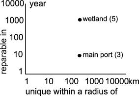
This diagram pre-supposes that in The Netherlands a main port is unique in a radius of some 300 km, but may be built in 10 years. Wetlands are unique on the same scale, but are only replenishable in a period of 1000 years. The logarithm of the product (the sum of the zero's) is respectively approximately 3 and 5.
27.16 Scenario development
With emphasis on possibilities, likelihoods or desirables, the builders of a scenario should have access to a wider field of creativity, expertise or actor-orientation than with more causally driven planning. The following means are at disposal.[17]
|
|
|
Figure 20 Foresight triangle |
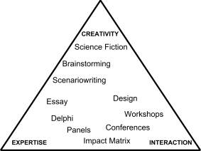
For further explanation we refer to the literature. An example of the Delphi Method is discussed in this book on page . The method comprises questioning a group of experts and confronting it quickly with the outcome, so that they might consider again. Next they are interviewed again, so that they may get an idea to what extent the group is going to support views. This usually leads to a convergence of ideas.
The cycle may be repeated several times, until the outlines of a scenario manifest themselves.
27.17 Limitation shows the master
Just very large-scale examples have been given here, since they feature a relatively small number of exogenous variables: by the same token they supply, with a grain to match, broader models which are, however, more appropriate for explanation. In the daily practice of study the scenarios of CPB, SCP, RIVM and AVV are usually regarded as given entities; that applies also for the population prognosis of the CBS. With a fitting amount of modesty study then tries to state something in the range of the first 5 years, 10 years at the most. Such a ‘forecast’ generates subsequently annual verification of the results (monitoring).
Perhaps
the impression is created here that the study challenges the position of the
Creator Himself. In the examples as practice generates them, much more is
already determined or given. One just looks at a limited number of variables on
a rather narrow time-horizon. As already mentioned in the start of
paragraph 1.13, usually scenarios are not meant to be forecasts, but tools to
facilitate and improve social and political discussion and decision making.