24 Mathematical Models

Taeke de Jong, R.P. de Graaf

24.1 Origins.................................................................... 2

24.2 The mathematical model is no reality...................... 2

24.3 Mathematics is the language of repetition.............. 3

24.4 Numbering(serial, sequence)................................. 3

24.5 Counting................................................................. 3

24.6 Values and variables............................................. 4

24.7 Combinatorics........................................................ 5

24.8 Taming combinatorial explosions........................... 7

24.9 The programme of a site........................................ 8

24.10 The resolution of a medium.................................... 9

24.11 The tolerance of production................................. 11

24.12 Nominal size systems.......................................... 12

24.13 Geometry............................................................. 18

24.14 Graphs................................................................. 20

24.15 Probability............................................................. 25

24.16 Linear Programming (LP)...................................... 27

24.17 Matrix calculation................................................. 29

24.18 The Simplex Method............................................. 30

24.19 Functions............................................................. 32

24.20 Fractals................................................................ 32

24.21 Differentiation....................................................... 33

24.22 Integration............................................................ 34

24.23 Differential equations........................................... 37

24.24 Systems modelling............................................... 38

A curriculum in mathematics for the Architecture Faculty at Delft University, taught for a few years during the nineties by the Mathematics Faculty, was ill-suited to the architecture staff, including its examples and references. So, the students who could not understand what use it was, experienced more nuisance than stimuli while designing, and were avoiding mathematics in the curriculum as a whole, where other disciplines could compensate for low grades in mathematics. The practice of design was doing well with high-school maths with some extensions, so why bother?

The realistic production of form is, as always, superior to the abstract mathematical detour via form description by Cartesian co-ordinates, even if fractal forms are generated. The mathematician and designer Alexander has been more successful with his ‘Pattern Language’ [1] than with his ‘Notes on the Synthesis of Form’.[2] The remainder of mechanics and construction physics is being taken care of by specialised consultant agencies and computers following delivery of a sketched design. No senior designer has any recollection of the content of mathematical education (s)he was exposed to during the sixties and seventies, when it was compulsory, while the practice featured nothing that might benefit from remembrance.

Of the lecture notes on architecture, ‘geometry’, ‘graph theory’, ‘transformations and symmetries’, ‘matrix calculation’ and ‘linear optimising’, ‘statistics’, ‘differential and integral calculation’ composed and, in the nineties, introduced in a simple form with the problem-orientated education only the latter may be found in the Faculty’s bookshop anno 2002. This last relict is due to the tenacity of the sector Physics of Construction. During the more mature years of building management matrix calculation for optimising exercises is being brushed-up from high-school maths. Then one is lacking the lost foundation in the first year. With the slow filtering-through of end-user friendly computer applications, as there are spreadsheets and CAD (pixel and vector presentations of form) during designing a new interest is dawning. Computer programs like Excel, MathCad, Maple or MatLab do ease experimenting with mathematical formulae as never before.

From these mathematical ingredients, also adopted by Broadbent[3] as relevant to architectural design, Maybe a new mathematics for architecture might be composed. Architecture itself and civil engineering, it should be remembered, were standing at the cradle of mathematics. This Chapter does not pretend to stand at the birth of a new building mathesis. As urban architects, its authors fall short of the proper attainments. However, it gives a global survey of mathematical forms that may be employed in architectural design – with a reading list – providing linkage with a new element as a point of departure: combinatorics. Whoever wants to brush up on high-school maths[4] or to get a bird’s eye view of mathematics as a whole[5] is referred to publications pertaining thereto. Experimenting with the Excel computer programme is especially recommended. In spite of that, Euclid’s answer to the question whether there would not be a simpler way to study geometry than his ‘Elements’[6] is still applicable: “There is no regal road to geometry’.

24.1 Origins

Mathematics is a language developed in order to describe locations, sizes (geometry), numbers (arithmetic)[7] and developments from observations (measurements and counts), to process these descriptions and to predict new observations on that basis. In this vein, until 500 BC, for the founding of cities in Greek colonies a square of 50 x 50 plethra (a ‘plethron’ is some 30 metres) was paced off thanks to a diagonal of 70 plethra, in order to realise straight corners.

Figure 1 Pythagoras

Pythagoras (580 – 500 BC) – or one of his pupils – next provided the well-known proof that the ratio should be slightly larger than 7 to 5; while the square of 7 is just one unit less than 25 + 25. From the womb of geometry, thus, the arithmetical insight was born that real numbers RR exist – such as the square root of 2, or the real length, derived therefrom, of the diagonal – not to be attained by simple partitioning (rational, QQ) of natural numbers (NN = 1, 2, 3 …). Geometry – literally: ‘measuring of the land’ – owns its first described development to the annual flooding of the river Nile. In ancient Egypt, floods wiped out the borders between estates and property, so that each year it had to be determined geometrically who owns what; as seen from standpoints which were not flooded. Arithmetic has roots in Phoenician trade. The Greek Euclid (around 300 BC) collected knowledge in both senses of his day and age in his book ‘Elements’, (via the Arab world) the cornerstone of all education in geometry well into the twentieth century. Euclid used earlier texts, but derived as the first the propositions of geometry by logical reasoning from 5 axioms.[8] With this, a process was completed emancipating mathematics from empirical practice of measuring and counting examples.

24.2 The mathematical model is no reality

Since then, mathematics can, like logic, without observing the sizes of input (non-empirically, a priori) come to new forms of insight (synthetic judgements). Logical proof dominating, they are accepted as new insight also without observing sizes of output. The philosopher Kant (1724 – 1804) struggled with the question how that is possible at all: synthetic judgement a priori.[9] For an empirical-scholarly theory always states that in the case of an independent observation from a set X, a corresponding independent observation from a set Y follows. If the elements of X and Y may be put in a corresponding, following, order so that they form the variable x and y, one may interpolate observations that have not been performed, while at constant conditions (ceteris paribus) – not included in the model – extrapolating to the future. A regularity of their correspondence is regarded as a working between them: y(x). Probable (causal) as well as possible (conditional) workings exist. If, for instance, the size of the population (x) is increasing, the number of buildings (y) is increasing as well following a hypothetical working y(x).

The larger the number of observations (n), the more convincing the theory. If one can demonstrate, by way of one hundred time sequences[10] (n = 100) that between the two of them a working (function) may be defined that convinces more than one single correspondence in the past year (n = 1). At larger numbers of independent input observations, the scholar can look for a mathematical working y = f(x) (e.g. y = ½ x) producing the same results as dependent observing (modelling). A just input and output must show a perceptible relation to reality, not the mathematical operations employed by way of a model. Different (mathematical or real) workings (functions) may yield the same result. As soon as other facts are observed than those predicted, the empirical theory is rejected; not necessarily the mathematical discourse playing a rôle therein; although the two occasionally get confused. If the predictions are confirmed, in its turn, the mathematical working model is often regarded as ‘discovered’ reality (‘God always calculates’)[11]. However, this is not necessary in order to accept a theory (until the opposite has been proven).

24.3 Mathematics is the language of repetition

Just as in daily parlance, in logic and mathematics as well, concepts (statements, expressions) are used and composed into a model (declarations, sentences, full-sentence functions[12], workings, functions) with operators like verbs and conjunctions. Logic is using these operators particularly in the case of conjunctions (for instance: if P, then Q) mathematics the verbs (functions such as adding and summing). Logical deductions in mathematics usually have the logical linguistic form: ‘if working P, then working Q’. However daily parlance has the capacity to name unique performances. This primal declarative function of everyday language has the character of a contract. Only when the performance has been witnessed anew is there a rational ground to start counting. What is repetitive is food for mathematics. For all mathematical operating, name-giving, as in everyday language, is – usually implicitly – pre-supposed. However, mathematics is of no use in unique performances. If one stone weighs one kilogram, then two stones weigh only two kilograms if they are ‘equal’. This equality (here in terms of size and material) can only be agreed on by normal words. Sub-dividing dissimilar stones in equal fragments (transforming sizes in numbers, analysis) can make unique specimens elective for counting, and then for mathematical operations based on that counting. The question whether that can be done will always remain; as in Solomon’s judgement: two times half a child means no child anymore. In analysis a connectivity, incorporating the essence of the architectural object, may get lost and will remain lost during synthesis to a different magnitude (counting). The scale paradox may be a nuisance while sub-dividing an object again and again in increasingly smaller parts, in order to compose next from this a different order of magnitude or to predict it (infinitesimal calculation, differential and integral calculation). The other, lost properties – in a specific context – may be taken into account next in the formulae (increasing validation, see page ), but this is just shifting the problem.

24.4 Numbering(serial, sequence)

Numbering(serial) just pre-supposes difference in place, not similarity in nature. I can enumerate the total of different objects in my room (or letter them) in order to be able to see later whether I am missing something, but this numbering(serial) does not allow mathematical operations. In spite of the fact that they are mathematically greatly important, since ordered difference of place (sequencing) is crucial in number theory.[13] The number(serial) serves as a label, name, identification (identification number, ID number, or index, in the case of variables) that may prevent exchanging, missing and double counting. By the same token, it is impossible to calculate with these numbers, although ‘numbering(serial)’ is pre-supposed silently in the case of ‘counting’. Sequencing of numbers has in principle no other purpose than that it is staying the same, even if the numbered objects are changing later in place. The number stabilises differences in place ever witnessed as if on a photograph.

Nevertheless, the sequence, in which one is numbering(serial), often gets, in practice, a meaning (for instance: in the order of arrival), allowing conclusions. Although one is inclined to introduce with an eye on that some logic in a numbering (categorising), it is halted sooner or later, while numbering is incurring lapses or lack of space. At current capabilities of information processing, this is why it is advisable, for instance, to open in a spreadsheet a database next to the column with sequential identification numbers (always to be produced independent of the shifting row and column numbers!) new columns in order to distinguish categories on which one wants to sort. For the mathematics it is important that it is possible to number(serial) input and output numbers, to index, identify and retrieve from a database in a fixed sequence and combination. The number(serial) is the carrier of the difference of place in a database. A reliable database is carrier of differences in nature and place in the reality (not that nature and place itself). To ensure that an identification code will always be pointing at the same object it should be invariant during the existence of that object. Additionally it is not allowed to have meaning in terms of content, such as a postal code and house number combination, for this changes in the case of home-moving the corresponding ‘object’.

24.5 Counting

Observations can only be expressed mathematically if they are occurring more than once (in a comparable context) and may be harboured as ‘equal’ in any sense in a set. Only then can one count them. The equality pre-supposition of set theory and mathematics is sometimes forgotten, or all too readily dissolved, by analysis (changing scale by concerning smaller parts). In this way an area of 1000 m² can be measured by counting, but each square metre has in many respects a different value that makes the area found in itself (without weighing) meaningless. The equality pre-supposition can lead to mathematical applications without sense, when the set described is too heterogeneous qua context or object for weighing. In this vein I can count the number of objects in my room, but each and every mathematical operation on this number alone does not lead to useable conclusions. Some objects are large, others small, some valuable, others not; or not elsewhere. From the number I might perhaps derive the number of operations in case of moving home, but these actions will be differing in their turn with the nature of the objects. Still I can say: “If I throw away something, I have less to move.” If I throw away a moving box with that argument, I have less to move, but this has no relation anymore with the effort (larger without the box) of moving that may have fostered the argument. Mathematical modelling would be misleading here and requires a comparable context.

So: some equality in nature is already pre-supposed when it comes to counting. Curiously enough, a difference is also pre-supposed: when counting, I am not allowed to point at the ‘same’ object twice (double counting). The objects pointed at should differ! What this difference in identity exactly is, is left here undecided;[14] for reasons of convenience we call it ‘difference of place’, although this does not cover, for instance, the problems involved in counting moveable objects like butterflies on a shrub, mutually exchanging places. A number, or variable, therefore pre-supposes equality of nature and difference of place, even if that place is not always the same.

The equality in nature pre-supposed when it comes to counting does require the definition of a set (determining which objects we count or not). This definition is pre-supposing within the set defined equality, but at the same time to the outside difference with other sets. This paradox is explained elsewhere in the book as a ‘paradox of scale’ or ‘change in abstraction, see page . In addition the ‘nature’ is not possible to change during counting. It is not allowed to use one century for counting one basket of apples, since it is likely that after an age like that the apples will not exist anymore.

The difference of place pre-supposed at the moment of counting does require a unique indication of place (which objects were already dealt with or not yet). By the same token such an indication of place is pre-supposing distances between the places (intervals) or between their centres (core to core distance); if that would not apply they would not differ and be unique. The size of the places indicated (scale) should be equal to the one of the objects placed (extension); if that would not apply one place could contain several similar objects, pre-empting identification of the objects themselves. Rather paradoxically, difference of place (uniqueness) is also pre-supposing an equality of scale (unit or order of magnitude) in order to guarantee that uniqueness. An object without scale (a point) may still be identified by mutual intervals. If these are small enough, points may produce a line, a surface or a volume.

24.6 Values and variables

Therefore, we are counting by pointing at similar objects differing in their various places (in order to avoid double counting). Since that place may change, we make a snapshot, stating for the differences of place a randomly chosen, but fixed sequence, numbering(serial). To each indication a different name is given, number(serial). The final number is the number(quantity) or figure. Sometimes the sequence is of no importance, so that it is possible to restrict oneself to a uniquely identifying naming (nominal values). When the sequence imports, the values are termed ‘ordinal’. Next, when the intervals between the objects numbered are equal, we call the number an ‘integer’. This enables operations with interval-valuessuch as adding, subtracting, multiplicating and dividing, without the need to indicate, count or re-count the objects and their places. With this different counts may be predicted from certain counts, but the result may also be a ‘non-object’. By naming this outcome ‘zero’ according to a price-less discovery of the world of Islam, and even by extending it after boundless subtracting with ‘negative numbers’ calculating is not restricted to objects accidentally present.

This is opening the road to calculation without reference to existing objects. By taking zero for a point of departure with at both sides the same interval as between the other numbers, the distance of this zero point to two numbers can provide a relational number (rational value). This is the foundation for measuring. Sometimes this results in fractions, that may be expressed in ‘rational numbers’. If they are represented as points on a line of numbers, it becomes apparent that in between the numbers resulting from division of integral numbers still other values exist (real numbers). Ratios can also yield a relation between numbers of different kinds of objects (for instance inhabitants per residence: residential occupation). The set of values of one kind is called ‘variable’. Function theory tries to work out arithmic rules for predicting, from the development of one variable x, another variable y. It is often difficult to determine, whether x and y entertain also a causal relationship, or are just demonstrating some connection (correlation); for instance on the ground of a common cause, a third variable, or if a great many causes and conditions are at work.

Particularly in probability calculus chances and probability distinguishing between these various kinds of values is important.[15] Then large numbers of results of a process are taken into consideration and the chance of a few of them is calculated (event). Extreme values are occurring less often as an outcome of many natural processes than values in-between. As a measure for the distribution between the extreme outcomes the average and its mean, the median and the modus are used. The average of a large number of values can only relate to interval values or rational values. In the case of ordinal values, no average exists, but a median (as many outcomes with a higher as with a lower value). In the case of nominal values it is also impossible to calculate a median; then a modus can be used (the number of values occurring most frequently).

When a set of values X is now compared to a different set Y in order to find between both a correlation, various statistical arithmetic methods (tests) exist, depending on the kind of values representing X and Y:

	Y
X	Nominaal	Ordinaal	Interval & rationaal
Nominaal (dichotoom)	Kruistabel	Mann-Whitney	· Grote steekproef: t-toets/ANOVA · Kleine steekproef, Y normaal verdeeld: t-toets/ANOVA · Kleine steekproef, Y niet normaal verdeeld: Mann-Whitney
Nominaal (niet di-chotoom)	Kruistabel	Kruskal-Wallis	· Grote steekproef: ANOVA · Kleine steekproef, Y normaal verdeeld: ANOVA · Kleine steekproef, Y niet normaal verdeeld: Kruskal-Wallis
Ordinaal	n.v.t.	Rang-correlatie	· Rangcorrelatie
Interval & rationaal	n.v.t.	n.v.t.	· Grote steekproef: Pearson-correlatie · Kleine steekproef, X en Y normaal verdeeld: Pearson correlatie · Kleine steekproef, X en Y niet normaal verdeeld: rangcorrelatie
Table 1 Overzicht toetsen op paarsgewijze samenhangen tussen twee kansvariabelen X en Y[16]

In this the nominal values have been distinguished in dichotomous (yes – no) or non-dichotomous (multi-valueous).

24.7 Combinatorics

As soon as counting has been mastered, one may name on a higher level of abstraction the internal categories (k), pre-supposed to be homogeneous, and unique places (n) themselves; number and count them. Allocating over the available places the kinds and within it the number of kindred cases (p) is the subject of combinatorics. It is pre-supposed in numerical systems and, therefore, a fundamental root of mathematics. This way the number of possible arrangements of 10 names over 2 places equals 100, over 3 it is 1000. Due to the Islamic discovery the notation of large numbers by combination of cipher names has become simple and more accessible to calculations.

Combinatorics may also be regarded as a basic science for architectural designing. More generally, one may calculate the number of possible arrangements, without any restriction, of k categories over n niches as kn. When it is supposed that 100 different kinds of building materials (among them air, space) may be used on a site of 100m², with 1 mln inter,connecting allocation possibilities of 10 x 10 cm, this is yielding already in a flat surface many more design possibilities (100^1000000) than there are atoms in the universe (10¹¹⁰). The designer is travelling, so to speak, in a multiple universe of possibilities, where the chance of meeting a known design is practically nil. With this, to all practical purposes, infinite number of possibilities no rational choice is possible by taking them all into account. Also, when restricted by a programme of requirements, in which the units ‘space’ must be positioned in certain amounts in inter-connection, the number of possibilities is still practically infinite. The various mathematical disciplines passing muster in the following paragraphs as possibly relevant for architecture, are described there as rational restrictions of this number of possibilities.

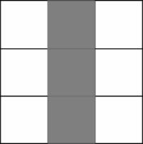
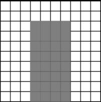
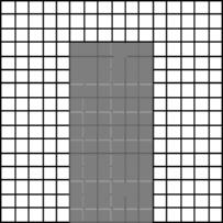
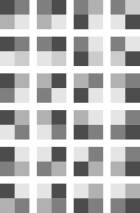
The designer, faced by a white sheet of paper or a blank screen, is asked to indicate on it difference in place (state of dispersion; form) and in kind (colour). The differences in nature are contained in a range to be generated (the 'legend', in its original connotation) spread in k units of colour (e.g. the programme) over n niches (appropriate fields, for instance on the grounds of the site); the differences in place.

n = 9 k=3, scheme

n = 100 k=32, rough draft

n = 256 k=78, Windows-icon

Figure 2 A programme, approx. 1/3 of the site, spread over the ground in 3 resolutions.

How many different states of dispersion can be generated in total? In mathematics the branch of combinatorics deals with that kind of 'arrangements' in finite sets and with counting the possibilities of arrangement under suitable conditions[17].

If a range of k = 3 colours is available for colouring n = 3 fields, 3³ = 27 variations apply. In this way the colours red, white and blue combined with three fields yield 27 distinct flags.

More generally: V(n,k) = kⁿ (variations with repetition). With as many colours as niches the expression reads nⁿ.

aaa	aba	aca	baa	bba	bca	caa	cba	cca
aab	abb	acb	bab	bbb	bcb	cab	cbb	ccb
aac	abc	acc	bac	bbc	bcc	cac	cbc	ccc
Figure 3 V(3,3) = 3^3 = 27 variations

Among them, however, there are many cases in which colours have been repeated or omitted. True 'tricolores' are but few. The first condition to be added amounts to the presence of all three colours. Colour one has 3 positions available; for the second 2 remain; and for the third 1. This limits the number of cases to 3 x 2 x 1 = 6, abbreviated to 3!, so-called permutations. More generally, one may write: P(n) = n! (permutations without repetition).

niches n	just as much different colours as niches
1	a
2	ab		ba
3	abc	acb	bac	bca	cab	cba
Figure 4 P(n) = n! : 1, 2 en 6 permutations

4	abcd abdc adbc dabc	acbd acdb adcb dacb	bacd badc bdac dbac	bcad bcda bdca dbca	cabd cadb cdab dcab	cbad cbda cdba dcba
Figure 5 P(4) = 4! = 24 permutations

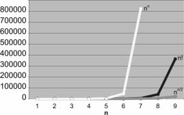
24.8 Taming combinatorial explosions

Permutations restrict the ultimate number of variations: 3!, is less than 3³; n! rises less fast than nⁿ, but faster than, for instance n^n/2, when only half the amount of niches is used for the number of colours ‘Factorials limit the largest powers’. Yet, permutations do increase fast enough to lead to a 'combinatorial explosion' on higher values for n:

Figure 6 Combinatorial explosions

How to select from all these possibilities? To many people this is a crucial question in personal life and in designing. With so many possibilities a conscious choice does not apply actually, so that during the reduction of the remaining possibilities, still not yet imaginable, one is guided by contingency, emotion of the moment, sensitivity for fashion, or routine. Deelder says: ‘Within the patches the number of possibilities equals those outside them.”; as long as the resolution is lowered.[18]

Although mathematics is used generally in order to arrive at singular solutions, where different possibilities are not taken into account to the dismay of the designer, this discipline may also be used to reduce the remaining possibilities within exactly formulated, but in other respects freely varying conditions (for instance a scale system of 30 x 30 x 30 cm)[19] and to survey them.

The branches of mathematics relevant to architecture are therefore seen here as the formulating of these restrictions on the total amount of possible combinations.

Systems of measure are mathematical sequences reducing the sizes of components to convenient sizes.

Geometry restricts itself to connected (contiguous) states of dispersion (shapes) such as lines, planes, contents, which can be described with a few points and with a minimum of information as to their edges.

Graph theory restricts itself to the connections between these points (lines with or without a direction) regardless of their real position.

Topology formulates transformations of forms and surfaces, so that one form can be translated in another one by a formula. This involves the direct vicinity of each point in the set of points determining this surface. For minimising the curved surfaces between the closed curves (soap skins) the forgotten mathematical discipline of the calculation of variances is necessary.[20] This mathematics is also applied to the tent roof constructions of Frei Otto. However, this discipline is too complicated to be introduced in this context.

Probability theory and its application in statistics restricts itself to the occurrence of well-defined events, for instance the happening of one or more cases among the possible cases in a given space or time.

Optimising by linear programming aided by matrix calculations formulates the remaining exactly restricted possibilities as the 'solution space’.

Next to these mathematical restrictions there are any number of intuitive restrictions causing the disregard of possibilities. If one recognises, for instance, in the illustrations on page 6 and following the image type of a door in a wall, the basis of the door (programme k) should lie in the lower part of the wall (the space present n), unless a staircase is drawn as well.

24.9 The programme of a site

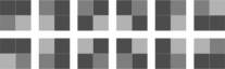
With variations (kⁿ) and factorials or permutations (n!) alone it is impossible to determine the number of cases when a particular colour has to be present in a predictable amount (a quantitative 'programme' per colour). With a programme for an available space n, where one colour (for instance black) has always to be present at least p times P(p,k) = n!/p! possibilities exist (permutations with repetition). The p! in the denominator of the ratio restricts the explosive effect of n! in the numerator at higher values of n, except of course, if it equals 1. That applies in the first column of the figure below; if p = 1 (so p! = 1) it has no effect on the ratio; the number of permutations P remains, as in the previous example with letters, 4! = 24. At p = 2 (p! = 2) and p = 3 (p! = 6) the number is restricted.

P(4,1) = 4!/1! = 24	P(4,2) = 4!/2! = 12	P(4,3) = 4!/3! = 4
Figure 7 Permutations in 4 niches, with at least k = {1,2,3} black elements combined with other hues.

The larger the programme p of one colour (in this case black) with regard to the total space available, the less possibilities remain for other colours to generate cases. Evidently, p, the number of colours surfaces to be distributed may not exceed the space n available.

The formula pre-supposes that the niches remaining will be filled with as many different colours. They generate the additional cases, not requiring attention from a programmatic point of view.

If not only the programme p, but also the complementary remainder n - p is combined into one colour, no other colours remain to generate additional cases. A permutation with two colours, p₁ and p₂ equals the formula n! / p₁!p₂! The possible arrangements of programme p1 and the remainder p2 develops into n! / p!(n-p)! (Newtons binomium)[21].

Within both surfaces, the sequence in which the niches are filled in with one colour is now irrelevant. The only consideration of importance left is the number of different instances in which one quantity p is allotted to n possibilities without a rôle for its own sequencing. This entity plays a leading part in statistics. Factor p then is the number of possibilities of an event, n – p is its complement of possibly not happening that event. So, not only possibilities in space apply: n may also reflect time. A little counter-intuitively the common expression is 'combinations'; and one simplifies the formula P (n, p₁, p₂ ) = n! / p₁! p₂! to C (n,p) = n! / p! (n - p)! ; or shorter still:

, 'n over p'.

(combinations without repetition).

C(4,1)	C(4,2)	C(4,3)
1x2x3x4/ ((1x)(1x2x3)) = 4	1x2x3x4/ ((1x2)(1x2)) = 6	1x2x3x4/ ((1x2x3)(1)) = 4
abbb,babb, bbab,bbba	aabb,abab,abba, baab,baba,bbaa	aaab, aaba, abaa, baaa
Figure 8 Combinations in 4 niches of 2 colours

Without fail, one will experience the highest level of freedom of design if a one-colour programme occupies half the site available (p1 = p2); a sound reason to plead with the principal for as much open space as space built.

At higher resolutions as shown in the diagrams on page 6 even the number of black-white combinations rises again explosively C(9,3) = 84, C(100,32) = 140 000 000 000 000 000 000 000 000 (1,4E+26 for short in Excel), the Windows-icon shown (16pixels x 16pixels = 256pixels), amounts at 78 black pixels C(256,78) already to 1,2149E+67 images. Excel calculates this with the command = COMBIN(256,78).

Again, the greatest freedom to design is found in an equal distribution between black and white pixels: C(256,128) = 3,50456E+75. If 256 colours can be used the variance formula is 256²⁵⁶ (10⁶¹⁶ or 2²⁰⁴⁸). This exceeds the number of atoms in the universe by far (10¹¹⁰ or 2³⁶⁵).

If one studies, for instance, 5625 locations of 1 km² in the colours 'built' (815) and 'open' (4818), approximately 10¹⁰⁰⁸ or 2³³⁴⁹ alternatives exist for the present 'Randstad' area in the Netherlands. The average PC cannot deal with this. Excel digests in this case at great pains p=156.

In this sense the designer is travelling in a multiple universe of possible forms (states of dispersion). The chance one runs into a known form is, in this combinatorical explosion, negligible

The number of elements of the programme (legends units, colours, letters) may be raised above 2; within the total sum of n, of course.

This enables the calculation of the numbers of cases belonging to a specified programme on a location. If one wants to allocate for instance 4 programmatic elements to n fields, there are

P(n,p₁,p₂,p₃,p₄) = n!/p₁!p₂!p₃!p₄! design possibilities. The total of the colour surfaces p₁+p₂+ … desired is again not allowed to exceed, of course, the surface available in total n. With a computer programme such as Excel one can calculate, for instance, that the possibilities of allocating 4 types of usage of 25m² each to an area of 100 m2 is 2,5E+82.[22]

24.10 The resolution of a medium

A pen, pencil or ball-point draws points and lines occupying a minimal surface, corresponding with the thickness of the material. Surfaces may then be depicted by filling in the surface with such lines. A computer screen is building an image from tiny surfaces (picture elements, pixels) that suggest contiguous lines or surfaces. This resembles the difference in the history of art between the Florentine (line-orientated) and the Venetian (point-orientated) ‘disegna’. A usual screen features 1024 x 768 pixels.

A pixel-orientated program (paint- or photoprogram) just supports the colouring of these points like in painting. If a ‘line’ or ‘surface’ is over-written, the only way to restore it is to fill in the previous colour of the over-written pixels. More often than not foreground and background are not distinguished in layers allowing display layer by layer, or in combination.

A computer drawing program (vector program, drawing program or CAD) just takes together the essential points of a drawing into a matrix of co-ordinates and translates the drawing into pixels between these points as soon as it is activated. The pixels in between are not being remembered during storage, so that mass-storage space requires less space than a pixel image. In the case of an enlargement of the drawing or of a detail, the resolution adapts itself automatically, so that the lines are not blurred.

A vector is a matrix with one column (or row) that in the flat plane just needs two co-ordinates to be defined from an origin. In the figure below three vectors a, b, and b-a have been drawn. They illustrate the calculation rules that are of great service in drawing programs and applied mechanics.

Figure 9 Defining line segments by vectors

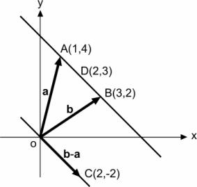
The line segment AB is represented by the co-ordinates of the vectors a and b; the points in between are calculated by giving a co-efficient I between 0 and 1 a sequence of values provided by the formula l (b-a)+ a.

vector substraction			l =0,5
A	b	b-a	l(b-a)	l(b-a)+a
1	3	2	1	2
4	2	-2	-1	3
Table 2 vector substraction and multiplication

This way I=0,5 yields the point in between D(2,3). The larger the number of values calculated, the greater the resolution of the line segment AB.

The combinatoric explosion of possibilities is already drastically reduced during the initial stage of the design by the coarseness or, in reverse, the resolution of the drawing. That is something different than the scale of a drawing.

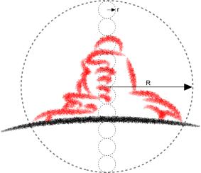
The position of a deliberately coarsely sketched line must be judged according to commonly understood conventions within certain margins. The size of such a margin surrounding a drawn point we call ‘grain’. We call the radius R of the circle inscribed in the drawing as a whole ‘frame’, and the ratio of the radius r of the grain to R ‘resolving capacity’, or ‘resolution’. The ‘tolerance convention’ could be interpreted as ‘any sketched point may be interpreted within a radius r, by that interpretation transforming the rest of the drawing accordingly’. The tolerance of the drawing is expressed by r.

Figure 10 The radius r of a grain here is approximately 10% of the radius R of the frame.

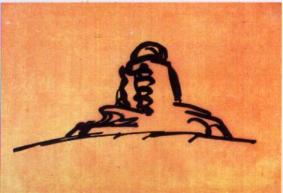
Figure 11 Sketch approx. 10% resolution

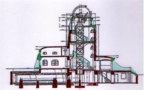
Figure 12 Drawing approx. 1% resolution

Screen approx. 0,1% resolution

source: http://aipsoe.aip.de/galerie/ausstellung/bilder

Figure 13 Mendelsohn (1920) Einsteinturm (Potsdam)

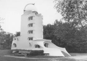
A sketch with a grain of roughly 10% of the frame is known as a loose sketch. It is used in an early concept, a type or a schema. It is often produced with a felt-tipped pen; with the same order of magnitude as the grain of the drawing, by that means stressing the tolerance convention. A ‘design’ hardly has a smaller resolution than 1%. A blue-print or computer screen does not exceed 0,1%. Only at this level things like details in the woodwork of a door and its frame in a wall are displayed. The total concept of a work of architecture is highly influenced by details, observed by the zooming eye of an approaching user.

24.11 The tolerance of production

A door should be slightly smaller than its frame in order to acquire a functional fit. In addition a carpenter or machine makes frames and doors respectively slightly larger, or smaller, than the nominal size written on the blue print.

This is also taming the mathematical use of positions behind the comma for architecture and technique in general. One is not allowed to think anymore in terms of numbers representing a point on the line of numbers: they are representing a margin, a band-with, a distance or class on that line. The nominal size is indicated on the blue-print, but it is certain that this precise size will never be delivered.

The frame should be equal or larger than the nominal size, the door should be smaller, but how much? The limits put to this product tolerance must be calculated by weighing the price of the precision and the performance of the door as a closure. If the tolerance of the frame opening is 0 to + 1mm, and the tolerance of the door –1 to –2 mm, the crack-width will be 1 to 3 mm, divided over two sides.

In order to decide whether to accept a batch of doors and frames or to send them back, no absolute measures are taken into account, but rather margins, classes such as ‘too small’, ‘small’, ‘large’ or ‘too large’. They may vary within limits of tolerance. In the case of the frames of the example in the above these limits are vis-à-vis the nominal size M:

‘too small’ < M + 0mm < ‘small’ < M + 0.5 mm < ‘large’ < M + 1mm < ‘too large’,

while for the doors the nominal measure

‘too small’< M –2 < ‘small’ < M – 1,5 < ‘large’ < M – 1mm < ‘too large’.

Figure 14 Acceptible and not acceptible sizes

In first instance one assumes that they are not too small, nor too large (zero-hypothesis, dotted contour in the drawing) while a few are measured in order to see whether they are belonging to these classes yes or no. However on the basis of a random selection one can refuse the batch frames and doors on false grounds (fault of the first kind) or accept them on false grounds (fault of the second kind). The first fault is a producer’s risk, the second fault consumer’s risk. Since two different risks apply, both faults can not be minimised by taking the minimum of their sum. For instance the consumer’s risk may be systematically smaller than what one may derive from the second fault. If the producer, for instance, is delivering systematically too large or too small frames and doors, one may settle for a smaller refusal. If both are within reasonable margins (too) large, they will still have an acceptable fit and width of the crack (above right in the following figure). This also applies for a systematic deviation to the smaller side (below left). Only when the frame is (too) small and the door at the same time (too) large (below right), or vice-versa (above left), does the sizing cease to be acceptable.

24.12 Nominal size systems

A restriction to multiples of 30 cm (little less than a foot) is a well-known bridle to sizes in construction of buildings. It reduces the combinatoric explosion of design possibilities. A grid like that is used to localise foundations, columns and walls without design efforts for smaller sizes. A grid may have a different size in any one of the three dimensions. A preceding analysis of usage may yield an appropriate size of the grid for a specific function. The distinct multiples of the size of the grid yield distinct functional possibilities. In the preceding paragraph a grid is implicitly used.

An arithmatical series has an initial term a, a reason v and a length n. The terms increase along a straight line by steps of v, starting with a. An example is the height of the first floor a of a building and its successors with a height of v, resulting in the series of heights h (normal dwelling and flat building[23], a=v₀):

	Normal dwelling		Flat building Van Tijen (1932)
n	v	h	v	h
9			2.85	27.15
8			2.85	24.30
7			2.85	21.45
6			2.85	18.60
5			2.85	15.75
4			2.85	12.90
3			2.85	10.05
2	2.6	8.0	2.85	7.20
1	2.6	5.4	2.85	4.35
0	2.8	2.8	2.70	1.50
				-1.20
Table 3 Arithmical series in building

Another example concerns a building with one oblique wall, like the KPN building by Renzo Piano in Rotterdam. The oblique wall commences on first floor level. The initial term is representing here the fixed surface per floor (supposed to be 100 m²). The n-th term indicates the surface at the level of the n-th floor. The sum of the terms is the total surface of floors at the oblique wall.

length	starting term	reason	array	sum
n	a	v	a+v*n
9			190	1450
8			180	1260
7			170	1080
6			160	910
5			150	750
4			140	600
3			130	460
2			120	330
1			110	210
0	100	10	100	100
Table 4 Arithmical sequence with sum

In these examples the reason remains equal, in the next example the reason changes each next n.

A sequence well-known from architecture and other arts is Fibonacci’s sequence: a new term equals the sum of two previous terms.

length	starting term	reason	array	ratio
n	a	v	a+v*n	r
9		3,4	8,9	1,62
8		2,1	5,5	1,62
7		1,3	3,4	1,62
6		0,8	2,1	1,62
5		0,5	1,3	1,63
4		0,3	0,8	1,60
3		0,2	0,5	1,67
2		0,1	0,3	1,50
1		0,1	0,2	2,00
0	0,1	0	0,1	1,00
		0	0,1
Table 5 Fibonacci’s sequence

The reason v is variable now, but the ratio r between two adjacent terms converges at last to the ‘Golden Rule’, ‘Golden Section’ or ‘Divine Proportion’: the smaller number (minor m) than has a fixed ratio to the larger number (Magior M). The Magior M, again has the same ratio to the sum of both:

m : M = M : (m + M).

From

follows:

For m = 1 follows for M/m and m/M:

and:

In the case of a geometrical series the ratio r is a factor of multiplication, so that the ratio of two adjoining terms is a constant.

length	starting term	ratio	array
n	a	r	a*r^n
9		2,000	51,20
8		2,000	25,60
7		2,000	12,80
6		2,000	6,40
5		2,000	3,20
4		2,000	1,60
3		2,000	0,80
2		2,000	0,40
1		2,000	0,20
0	0,1	2,000	0,10
-1		2,000	0,05
-2		2,000	0,03
-3		2,000	0,01
Table 6 Geometrical sequence

A geometrical series can be continued for negative values of n while the array remains positive for real architectural purposes.

Applications of geometrical series are found in the financial world, like in compounded interest and in annuities. An investment of € 1000,- at an interest of 5% yields after 1 year € 1000 * 1.05 = € 1050. After two years this is € 1050 * 1.05 or € 1000 * 1.05 * 1.05 = € 1102.50.

Experiencing sound is also an example of the geometrical series. An increase of sound to the amount of 10 dB is experienced as twice as loud; an increase of 20 dB as four times.[24]

For architectural applications most geometrical series are not very useful, because adding architectural elements next to eachother (juxtaposition) produces new sizes, not recognisable anywhere else in the series.

However, when we choose the Golden Section as a ratio we get:

length	starting term	ratio	array
n	a	r	a*r^n
9		1,618	7,60
8		1,618	4,70
7		1,618	2,90
6		1,618	1,79
5		1,618	1,11
4		1,618	0,69
3		1,618	0,42	▲
2		1,618	0,26	m+M
1		1,618	0,16	M
0	0,1	1,618	0,10	m
-1		1,618	0,06	M-m
-2		1,618	0,04	▼
-3		1,618	0,02
-4		1,618	0,01
-5		1,618	0,01
Table 7 Golden Section

Now, every adjacent pair of sizes is flanked by their sum and difference, just as in the non geometrical Fibonacci sequence. Adding and subtracting of adjacent terms do not produce new sizes.

The differences in use of both proportion rules are only visible in the smallest stages:

Figure 15 Fibonacci house & Golden Section house

Many attempts have been made to recognise the Golden Section in nature and the human body. Until 1947 Le Corbusier took the human length of 1.75 m as a point of departure. Later, he started at 182.9 (red array) and 2.16 m (blue array): the reach of a man with a hand raised as high as possible.

< 1947	Red array			Blue array
0,2	0,2			0,3
0,3	0,4			0,4
0,5	0,6			0,7
0,9	0,9			1,1
1,4	1,5			1,8
2,3	2,4			3,0
3,7	3,9			4,8
6,0	6,3			7,8
9,8	10,2			12,6
15,8	16,5	Modulor		20,4
25,5	26,7	27		33,0
41,3	43,2	43		53,4
66,8	69,9	70	86	86,3
108,2	113,0	113	140	139,7
175,0	182,9	183	226	226,0
283,2	295,9			365,7
458,2	478,8			591,7
741,3	774,7			957,4
1199,5	1253,5			1549,0
1940,8	2028,2			2506,4
3140,2	3281,6			4055,4
5081,0	5309,8			6561,8
8221,3	8591,5			10617,2
13302,3	13901,3			17179,0
Table 8 Measure systems of Le Corbusier

The red and the blue columns are featuring steps with a stride too wide between the terms for architectonic application. For this reason, Le Corbusier combined them and rounded them off in the Modulor. There are many other attempts in making the possibilities of the design with scale sequences easy to survey and well to maintain in the design decisions with a pre-supposed, built-in beauty.[25]

The problem of too large steps with the Golden Section was later solved by Reverend van der Laan. He selected the ‘plastic number’ r = 1,3247180 for a ratio. This is a solution of the equation r¹ + r⁰ = r³ as well as of the equation r¹ – r⁰ = r^r-4

Figure 16 Golden Section

Figure 17 Plastic Number

Since any number may be substituted for the initial term a, for instance another term from the series, the more general formulae rⁿ⁺¹+rⁿ=rⁿ⁺³ and rⁿ⁺¹-rⁿ=r^n-4 may be employed. In the row below this means that the formulae can be shifted, while keeping the mutual distance constant.

length	starting term	ratio	array
n	a	r	a*r^n
9		1,325	1,26
8		1,325	0,95
7		1,325	0,72
6		1,325	0,54
5		1,325	0,41
4		1,325	0,31	s
3		1,325	0,23	r^n+r^n+1=r^n+3
2		1,325	0,18
1		1,325	0,13	r^n+1
0	0,1	1,325	0,10	r^n
-1		1,325	0,08
-2		1,325	0,06
-3		1,325	0,04
-4		1,325	0,03	r^n+1-r^n=r^n-4
-5		1,325	0,02	t
Table 9 The plastic number

The sum and the difference between two consecutive terms are returning in the series as at the Golden Section, albeit 2 places upward or 4 places downward, rather than by 1 each time. Therefore they are forming with addition and subtraction no new measures while preserving the ratio r.

Figure 18 Morphic Numbers

Aarts et al. have demonstrated that this ratio is, next to the Golden Section, the only one with this property.[26] Together they are called ‘morphic numbers’.

24.13 Geometry

It is impossible to imagine a door distributed in tiny slits across a wall. Geometry restricts itself to contingent states of dispersion (lines, surfaces, contents) that can be enveloped by a few points, distances and directions. This pre-supposition of continuousness lowers the amount of combinatorial possibilities dramatically. The extent to which this geometrical point of view restricts the combinatorial explosion, is the subject of combinatorial geometry: it studies distributions of surfaces and the way these are packed.

However, the often implicit requirement that points in one plane should lie contingent within one, two or three dimensions is more obvious and self-evident in the case of a door, than in the one of a city. That is the reason why urban design is interested in non-contingent states of dispersion. The possibilities are restricted geometrically, following the often implicit pre-supposition of rectangularity. Particularly efficient production suggests this pre-supposition.

When one limits oneself to enclosed surfaces or enclosed spaces and masses, three simple shapes may be imagined in a flat plane: square, triangle and circle. Why are they so simple? They survive as geometrical archetypes in geometry and construction everywhere.

Minimal number of directions in one loop	Minimal number of changes of direction in one loop	Minimal variation of changes of direction in one loop
Figure 19 Simple shapes

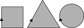
Their simplicity may be explained by the minima added in words to the diagram. This gives at the same time a technical motivation for application. A minimal number of directions is for production - e.g. sawing and size management - an effective restriction. Any deviation influences directly the price of the product. A minimal number of directional changes (nodes) is constructively effective (also from a viewpoint of stiffness of form). A minimal variation in directional changes(one without interruption, smooth) is effective with motions in usage; when one keeps the steering wheel of a car in the same position, a circle is described at last. They have been drawn in the diagram, with an equally sized area (programme). Their circumferences then are roughly proportioned like 8 : 9 : 7.

Our intuition meets its demasqué, by keeping the area equal: the triangle wins out. This visual illusion may be used for spaces needing particularly spatial power.

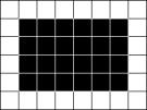
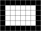
A second example of the capacity of geometry to lead to counter-intuitive conclusions about areas is the seeming difference in surface between the centre and the periphery as Tummers[27] emphasises. In the diagram below they equal one another.

Figure 20 Apparent difference in surface between centre and periphery

Functions characterised by the importance of inter-connectedness at all sides - like greenery, parks - tend to be better localised centrally, while differently structured functions (e.g. buildings) are better placed peripherally.

The triangle is playing an important rôle in geometry because all kinds of shapes on flat or curved surfaces and stereometrical objects may be thought of as being composed out of triangles. Measuring the surface, also on bent surfaces (geo-metry), is dependent on insight in the properties of triangles (triangulation) since it establishes a one-to-one relationship between lines and angles (trigonometry). In the measuring of angles (goniometry) next to the triangle the circle plays a crucial rôle. Descriptive geometry[28] makes images of three-dimensional objects on a two-dimensional surface (projections), so that they may be reconstructed eventually on a different scale. With this, descriptive geometry is a fundamental discipline for architecture and technical design in general; for this description enables in its turn a wealth of mathematical and designing operations. The triangle also plays an important rôle in the technique of projecting.

These subjects have already been described thoroughly and systematically by Euclid in his ‘Elements’ around 310 BC. Until in the twentieth century this book has been the basis for education in ‘Euclidean geometry’. The work is available on the internet with interactive images and it is still providing a sound introduction into elementary geometry, as always.[29] Together with the co-ordinate system of Descartes geometrical elements became better accessible to tools from algebra such as vectors and matrices (analytical geometry).

When objects can be derived with rules of calculation in a different way than by congruency, equal shape or projection, when they can be represented or shaped into another, ‘topology’ is the word. The properties remaining constant under these transformations – or oppositely change into sets of points – can be described along the lines of set theory or with algebraic means. This is leading to several branches of topology. What is happening during a design process, from the first concept via typing to design, is akin to topological deformation, but it is at the same time so difficult to describe, that topology is not yet capable of handling.

On the other hand, the existing topology is already an exacting discipline, pre-supposing knowledge of various other branches of mathematics, before the designer may harvest its fruits. Nevertheless, it is conceivable that a simple topology can be developed, restricting the combinatorical explosion of design possibilities rationally in a well-argued way, in order to generate surprising shapes within these boundary conditions. It would have to describe constant and changing properties of spaces, masses, surfaces and their openings in such a way, that complex architectural designs could be transformed in one another via rules of calculation. With this, architectural typology and the study by transforming design would be equipped with an interesting tool. The computer will play a crucial rôle in this.

When a design problem can be described in dimension-less nodes and connecting lines between them, graph theory could be a predecessor.

24.14 Graphs

When one notes in a figure only the number of intersections (nodes) and the number of mutual connections per intersection (valence, degree of the node) we deal with a graph.

A graph G is a set ‘connecting points’ (nodes, points, vertices) and a set of ‘lines’, branches (arcs, links, edges), connecting some pairs of connecting points together. A branch between node i and node j is noted as arc (i,j), shortened arc^i j.

Length, position and shape of the connecting points and branches are without importance in this. (In architecture the relative position of the connecting points vis-à-vis one another will probably be of importance.)

Among many figures corresponding types may be discerned wherein neither length nor area play a rôle (e.g. designing structure, not yet form and size). This enables the study of formal, technical and programmatical properties in space and time even before the sizes of the space or the duration in time are known.

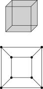
A cube may serve as an example. It has 8 nodes. Each of them has 3 connections. This fixes the number of connecting lines (branches) : 8 X 3/2 = 12. For each connecting branch occupies 2 of the 8 x 3 connections in total.

	input		output
figure	nodes	connections per intersection (valence, degree)	branches = nodes x valence/2	planes = branches - nodes+ 2	connections = branches x 2	boundaries = branches x 2	boundaries per plane (valence) = boundaries / planes
tetrahedron	4	3	6	4	12	12	3
cube	8	3	12	6	24	24	4
octahedron	6	4	12	8	24	24	3
K3,3	6	3	9	5	18	18	3,6
K5	5	4	10	7	20	20	2,9
Table 10 Nodes and connections in regular solids

Following the formula of Euler, the number of planes = number of branches - number of nodes + 2. As soon as the planes (still without dimensions) come into the picture, we deal with a map. By the same token it suffices to count in a figure the intersections and their valencies in order to be able to calculate the number of branches and planes in the map.

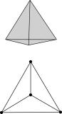
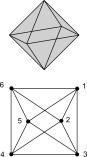
The regular solids can be represented in a plane by a graph.

tetrahedron	cube	octahedron
Figure 21 Regular solids as a graph

Based on this, the terminology of graph theory is readily explained. These are single graphs: there are no cycles arriving at the same node as the one of departure; or multiple connections between two nodes.

Furthermore, they are regular: in each node the number of connections per graph is equal.

The tetrahedron has a complete graph (K) unlike the other two, where possible connections - the diagonals - fail.

The graph of the cube clearly demonstrates that the outer area should be in calculated in order to count 6 planes. It is as if the cube is 'cut open' in one plane, in order to 'ex-plane' it on the page. It is immaterial which plane serves as outer plane. Graph theory does not yet distinguish between inside and outside.

The graphs of the tetrahedron and the cube are 'planar': the flatland does not feature crossings without intersection. The diagram below shows to the left an 'isomorph graph' for the octahedron where the number of nodes equals the number of valencies.

Compare the octahedron graph with the one of Figure 21.

octahedron	K5	K3, 3
Figure 22 Octahedron, K5, K3,3

The branch between nodes 6 and 1 of the octahedron may be 'contracted' in such a fashion, that one node remains, where all other branches end previously ending in 6 and 1, with whom they were 'inciding' or 'incident' in the parlance.

If a graph yields to contraction to K5 or K 3,3, it can be proven that it is non planar. Architectonically this is especially important: by the same token no blueprint can exist that relates all the relationships as recorded in the graph.

4 rooms	diagonal	K4
Figure 23 Four connected rooms

According to K4, each of the four rooms, may be linked by 3 openings mutually among themselves. The left shows the solution with two openings where one may circulate. The corresponding graph (a circuit) has also been drawn. The middle one demonstrates a solution where only two of the four rooms have 3 doors. To solve the complete graph K4, a ‘dual map’ must be drawn. To do that, K4 is made isomorphically planar, and the planes are interpreted as ‘dual nodes’. The outer area of the graph is involved as a large, encircling dual ‘node’.

These dual nodes (white in the drawing below) should be connected in such a way by dual branches (dotted lines) that all planar branches will be cut through just once:

Isomorphic planar K4	Dual K4 with doors	An architectural solution
Figure 24 Dual graph

These cuttings through have become ‘doors’ (or windows) in the dual graph. The dual lines are ‘walls’ of a dimension-less blue-print and the dual points are constructive inter-connections. If this prototypical blue-print is regarded as ‘elastic’, it can be transfigured in an isomorphic way into a design, by giving the surfaces at random forms and shapes. Type K4 is usual for bathrooms and museums.

From a fundamental point of view, no solution exists in flatland for 5 rooms, each sharing one door with all other rooms (K5): no planar graph could be drawn of K5.

By regarding each space firstly as a node between other spaces, the design possibility of programmatic requirements can be verified along the lines of graph theory. Suppose, that the programme of relations between rooms in a dwelling results in the following scheme:

Figure 25 Possible relations between rooms

This graph demonstrates that a third bedroom (10) can not be connected to the bathroom if it is already connected to the hall (1) and the garden (6). When the requirement that all bedrooms should give to the garden is skipped (the connection 9-6), a solution exists in which all bedrooms give access to the bathroom.

At 10 rooms, combinatorially speaking 10!/2!8! = 45 relations exist (K10). They can never be established directly (made planar):

K10	Planar selection
Figure 26 Planar selection of possible relations

Yet, the selection of the relational scheme can be made planar, therefore, it has a solution. With their high valence (number of doors), the hall (1) and the garden (6) are crucial. If these nodes are removed, a ‘non-conjunctive’ graph originates. Following that, it may be decided to give the rooms 6 to 10 a separate floor; or even its own location. If a node alone allows this freedom, it is termed a ‘separational node’ The minimal number of nodes n that can be taken away with the incident branches in order to make them non-conjunctive makes the graph ‘n-conjunctive’. It is an important measure of cohesion in a system. In the figure following possible realisations are given by drawing the dual graph:

Planar + dual	Dual+doors
Solution 2 wings	Solution 2 levels
Figure 27 Different solutions of the same dual graph

A map of the national roads of our country is an example of a network. Each branch is denoting a stretch of road, each node a crossing or roundabout. By supplying branches with a length the user can determine quite simply the distance between his point of departure and that of his destination. If the traffic streams across the network and their intensities are known it is easy to determine the traffic load on each branch. A network like this may also represent the traffic deployment within a building, where the branches stand for corridors, stairs and elevators. Then it can be determined, for instance, how many students change places in between classes in the building. This gives a basis for deciding on dimensioning the corridors e. t. q.

The organisational structure of an enterprise may also be depicted in a network. If this structure should be expressed in the building at the design of a new office, this network may form a point of departure; one may derive from it which departments are directly linked to one another with the wish to realise this physically in the new building.

By the same token networks enable the structure of a building or an area, without describing the whole building or the whole area.

A graph with a weight (stream, flow) of any type (time, distance), on its branches, is called a network.[30] If this flow displays a direction as well, the network is termed a directed graph. A path is a sequence connecting branches with a direction and a flow. A network is a cyclical network, if a node connects with itself via a path. The length of the path is determined by the sum of the weight of the paths concerned. The length of the shortest path between two nodes may be determined by following, step by step, a sequence of calculating rules, the shortest-path algorithm.[31]

An algorithm in this vein exists for the longest path, the 'critical-path method'. This method is used in 'network planning' in order to determine, within a project, the earliest and latest moments of starting and finalising each and any activity of the project; and, consequently the minimal duration of the project.[32] In this, the nodes represent the activities, the branches the relation between the activities.[33] The start of an activity (successor) is determined by the time of finalisation of all preceding activities (predecessors). With regard to the network planning, it is feasible to monitor the progress of (complex) projects; as well as to survey the consequences of retardation of activities. However, the problems caused by retardation are not able to be solved. In order to achieve such a solution one has to employ other techniques; like linear programming (LP).

24.15 Probability

An event is a subset of results A[34] from a much larger set of possible results W[35] (a set much larger) that might have yielded different results as well. The chance of an event of A well-defined instances taking on ''what had been possible'' W is - expressed in numbers - A/W. Often it is not easy to get an idea of what would have been possible; certainly when W has sub-sets dependent on A, for the event may influence the remaining possibilities.

Say, that the number of possibilities for filling in a surface with 100 buildings from 0 to 9 floors is 100¹⁰. Two of these possible events have been drawn below: an example of ‘wild’ and one of ordered housing. The chance that with a maximal height of 9 floors one of the two will be realised exactly is 2 in 100¹⁰ (summation rule).

Figure 28 Wild and ordered housing

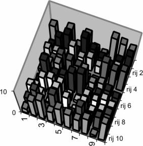
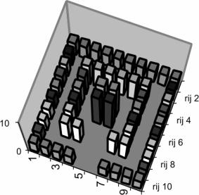
The wild housing leaves the elevation of a building completely to contingency. As a consequence in 100 buildings the average elevation is approximating the middle of 4,5 between 0 and 9. The average of 2.2 floors of ordered housing is deviating more from the mean than the one of wild housing and, therefore, less ‘probable’. In the matrix below the elevations from the drawing of the wild housing have been rendered.

columns rows	1	2	3	4	5	6	7	8	9	10	mean per row
1	5	0	6	1	6	2	1	8	7	6	4,2
2	1	5	7	2	8	5	3	1	4	7	4,3
3	3	3	3	7	4	5	3	1	5	1	3,5
4	2	3	6	5	4	0	0	9	7	8	4,4
5	1	6	6	1	5	7	3	4	2	0	3,5
6	0	9	5	6	8	9	2	3	6	4	5,2
7	1	6	7	6	2	1	5	4	6	4	4,2
8	5	3	0	8	5	0	6	3	5	8	4,3
9	3	8	1	9	0	3	8	4	6	9	5,1
10	2	7	9	5	8	7	6	8	1	9	6,2
Average for the total:											4,5
Table 11 An average of means

It is as if a dice with ten faces has been thrown one hundred times. The rows form every time a sample of 10 ‘throws’ from the 100. Such a partial event in the first row of buildings can already yield 10¹⁰ (10 000 000 000) averages with only 10! = 3 628 800 different averages (less than 0,4%!). If one studies from among them all the 10 averages comprising the natural numbers ( 0 to 9) one must conclude that for 4 and 5 the maximum of possible combinations exist (9!/4!5! = 126).

rows													mean per row
9!/0!9!=	1		0	0	0	0	0	0	0	0	0		0
9!/1!8!=	9	combinations for the mean										1
9!/2!7!=	36	combinations for the mean										2
9!/3!6!=	84	combinations for the mean										3
9!/4!5!=	126	combinations for the mean										4
9!/5!4!=	126	combinations for the mean										5
9!/6!3!=	84	combinations for the mean										6
9!/7!2!=	36	combinations for the mean										7
9!/8!1!=	9	combinations for the mean										8
9!/9!0!=	1		9	9	9	9	9	9	9	9	9		9
Average for the total:												4,5
Table 12 Possibilities to compose averages from the 10 numbers from 0 to 9 an average

In order to get any other average a lower number of combinations is available. For a result of an average of 0 or 9 , for instance, just one thinkable combination exists (the improbable events of 10 zeroes or 10 nines. The averages are condensing themselves between 4 and 5. The combination possibilities of the above are representing this way the chance density. In the column in question a Gaussian curve is, therefore, manifesting itself.

Obviously, this applies to the columns (events) as well. In the table below the mean, median and mode of the columns are cumulatively rendered by taking each time more columns into account.

n =	10	20	30	40	50	60	70	80	90	100
mean	2,3	3,6	4,1	4,3	4,4	4,4	4,3	4,3	4,4	4,5
median	2,0	3,0	4,0	5,0	5,0	5,0	5,0	4,5	5,0	5,0
modus	1,0	3,0	3,0	5,0	5,0	5,0	5,0	5,0	5,0	5,0

The larger the number of throws, the closer the average approximates 4,5. However this does not apply as yet for the median (as many results above as below) and even less for the mode (the highest result). Their deviations of the mean are indicating asymmetrical, skew distributions.

Figure 29 More results stabilise the mean

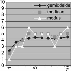
The mean reduces the variation of a large set of numbers to one number. The variation itself is then very partially acknowledged with the ‘standard deviation’ sigma (σ). Some 2/3 of the cases differ usually less from the mean than this standard deviation. Some 95% lies within 2 x σ from the mean (95% probability area). This gauge σ only makes sense in the cases condensing themselves by combination possibilities around a mean. This is not applicable, for instance, for the individual cases of the example above. They have each an equal chance for 0, 1, 2, 3, 4, 5, 6, 7, 8, or 9 floors. The mathematically calculated ‘standard deviation’ on this basis would amount to some 5 floors at each side of the 4,5 . Within this wide margin, not carrying meaning, all results are falling; not just the two thirds of them. However, the 10 columnar averages do concentrate themselves at the total average; for from average values like 4 and 5 more combinations of individual elevations could be composed than from extremes such as 0 or 9. If we consider the spreading of these 10 more ‘obedient’ outcomes, then the standard deviation may be calculated from the sum of the outcomes (sum of outcomes) and the sum of their squares (squared sum):

Column-number	1	2	3	4	5	6	7	8	9	10	sum
outcome (means)	2,3	5,0	5,0	5,0	5,0	3,9	3,7	4,5	4,9	5,6	44,9
square	5	25	25	25	25	15	14	20	24	31	209,8
Standard deviation s = ROOT((sum of squares – sum of outcomes^2/n) /n) n=10											0,91

The standard deviation is here σ = ROOT(squared sum – sum of outcomes ^2/n)/n) = 0,91^[36]. Mean μ as well as standard deviation σ may be used for the comparison of the event in the bar graph with a corresponding normal distribution (μ,σ) of the chance density that is approached in the case of very many events. This distribution represents the total of probable possibilities Omega Ω at a given μ and σ against a back-drop from which the event A is one outcome.

Figure 30 Classes of observations

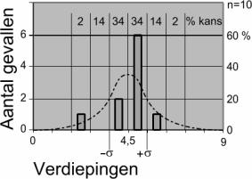
At both sides of the average with a sigma of 0,91 floors five classification boundaries have been distinguished with 0 and 9 for extremes. The number of cases between 4.5 and 5.4 floors is above expectancy.

Table 13 Chance within class boundaries

Employing classification boundaries in this manner it may be seen at once in how far these results could have been expected on the basis of a normal distribution of chances. The case of a columnar average of just 2,3 floors (in the left column of the wild housing area) is rather far removed from the total average. Each average number of floors under 2,7 or above 6,3 lies outside the 95% probability area (14+34+34+14 = 96).

Now the usual mistake of policy makers and statisticians is neglecting these cases; or even using them as a point of departure for establishing norms. Contrariwise the designer is specialised in improbable possibilities from the available combinatorial explosion of possibilities, albeit within a context ruled by probabilities.

24.16 Linear Programming (LP)

Imagine we want to invest on a location of 14.000 m² within 16 months in as much housing (D units) and facilities (F units) as possible: ^[37] (see also page )

asked: number of units	mln Dfl investment	1000 m^2surface	months building time
	per unit
D	5	2	1
F	8	1	2
maximize	Z	14	16
Table 14 LP problem

What to build? In other words: what are F, D and Z? The objective (Z maximised) implies making 5D + 8F as large as possible (maximising it) under the following boundary conditions: (also known as restrictions or constraints)

Max! Z=	5	D	+	8	F	(maximize this investment Z within
	2	D	+	1	F	£	14	x1000 m^2 surface and
	1	D	+	2	F	£	16	months, while
					F	³	0	f and d are not negative)
		D				³	0
Table 15 LP operationalisation

Figure 31 Solution Space

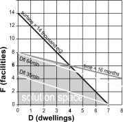
All points (combinations of D and F) within the solution space satisfy all constraints, but not all fulfil the requirement of optimisation of a maximal Z. When no facilities are to be built (F=0) the surface restriction 2D+1F £ 14, determining the maximal value of Z, is restrictive, resulting in D = 7 dwelling units to be built in 1D + 2F = 7 months. The investment will be 5D + 8F = 35 mln. If no dwellings are to be built (D = 0), the maximum duration of building becomes the limiting factor, realising 8 units of facilities within 16 months. The maximum investment Z would be 64 mln. This is not yet maximal. Considering only the surface constraint, F = 14 units of facilities could be built on the site resulting in an investment of 112 mln, but that would take too much time: 28 months.

Next, we want to know for which point within the solution space the investment represented by the function 5D + 8F, is maximal.

In the origin (D=0, F=0) the investment will be zero, so Z = 0. Moving the line to D > 0 and/or F > 0 will increase Z. We will find the solution after moving this line as far as possible from the origin without leaving the solution space. In this case this point (4,6) The investment will be 5 * 4 + 8 * 6 = 68. The lines through this point define the solution. The boundary conditions are then called 'effective'. Removing or changing one of the boundary conditions will amount to changing the solution. Were there, for some reason, 15.5 months available, we could realise 4.2 dwellingunits and 5.7 facilityunits. If a feasible solution has been found, the solution will always find itself in a corner point (intersection of two lines); unless the object function (objective) is parallel to the boundary condition determining the solution.

This simple example already shows how sensitive optimisations are vis-à-vis their context (two weeks less building time results in a different solution) and how important it is to re-adjust continuously the boundary conditions, which are quickly considered stable, or to vary them experimentally in sensitivity-analyses with regard to different perspectives, changing contexts. This requires tireless calculation in order to be able to react to changing conditions. If such boundary conditions are within one's own sphere of influence they may also be considered as objectives. This way the choice of what is called an end or a means gets a different perspective.

Often designers manage to annihilate boundary conditions deemed stable: suddenly, different objectives become interesting. This sensiti-vity with regard to context only increases, if more boundary conditions or objectives are taken into account; for instance, the valuation of occupants of facilities (e.g. 3) in contrast to dwellings (5) : then maximize 3F + 5D, while keeping, for example, the budget constant. The solution space now has 5 rather than 4 corners, which might be more optimal in one way or another.

With a problem with n variables and m restrictions, the cornerpoints number m+n / m!n!.

In case of a LP problem with 50 variables and 50 restrictions some 10 ²⁹ equations must be solved. That is a time-consuming task even for the fastest computer. Luckily, it is not necessary to study all corner points. Proceeding from an initial solution obeying all conditions (and admitted or feasible solution) far fewer corner-points have to be investigated in order to find a solution; approximately m+n. The procedure to follow is known as the Simplex method (see page 30), that finds an eventual solution in a finite number of steps. With this the inequalities are transformed into equalities by adding 'slack variables' or ‘remainder’ variables before the inequal sign:

2D + 1F £ 14	becomes	2X1 + 1X2 + X3 = 14
1D + 2F £ 16		1X1 + 2X2 + X4 = 16

This way unknown variables have been added. With two of them, such as F and D, optimisation can still be visualised on a piece of paper. If more than two dimensions of decision are to be made variable, one is restricted to the outcome of an abstract sequence of arithmetical operations like the Simplex method, a method employing matrix calculation.[38]

24.17 Matrix calculation

Take a system of equations, for instance:

2x₁ - 3x₂ + 2x₃ + 5x₄ = 3

1x₁ - 1x₂ + 1x₃ + 2x₄ = 1

3x₁ + 2x₂ + 2x₃ + 1x₄ = 0

1x₁ + 1x₂ - 3x₃ - 1x₄ = 0

---------------------------------------------------

a₁x₁ + a₂x₂ + a₃x₃ + a₄x₄ = b

Usually the co-efficients, the unknown variables and the results are symbolically summarised as Ax = b. In this A, x and b represent numbers concatenated in lists (matrices) or columns (vectors) [39], in this case

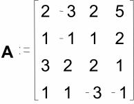
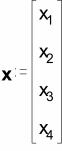
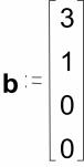
This way the sum of the products 2x₁ - 3x₂ + 2x₃ + 5x₄ equals the first number of b (b₁ = 3), the next one 1x - 1x₂ + 1x₃ + 2x₄ equals b₂ = 1, etc. This shows how matrix multiplication of each row of A with the column vector x works. In the imagination the column must be toppled in order to match each a with its own x. In order to calculate such a sum of products at all, the number of columns should of course, be equal to the number of rows of x. Considering that the number of rows of A conversely is not equal to the number of columns of row vector x, vector multiplication xA is impossible here: in matrix calculation Ax is not the same thing as xA. One cannot divide matrices and vectors [40], but often it is possible to calculate an inverse matrix A^-1, so that one may write Ax = b as x = A^-1b [41]. By that, one can not only determine n unknown variables in n equations by substitution, much writing and many mis-calculations, but also by applying the Gauss-Jordan method; or in the case of more solutions b by the (inverse matrix)

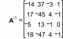
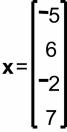
The point of contact of the two equations of paragraph 24.16 may be determined easily both graphically and by substitution, but in the matrix guise the solution would look like this:

Matrix A can also be used for calculation of the area and number of times needed to realise any combination of number of dwellingunits and number of facilityunits. If we want to know how may units can be realised within a given area and time, we have to solve the problem x = A^-1 b. In real life the number of variables and constraints are not equal. Neither is it necessary to consume all available space and time. So inequalities will be introduced. The result is that the number of solutions may be infinite. Therefore the linear objective-function has been added. Among all solutions find that one that results in a minimum or maximum value of the objective function as shown in 24.20.

The essential operations, with regard to the solving of a system of equations by means of the Gauss-Jordan method are:

· multiplying all co-efficients of one row with an identical factor adding a multiple of a row to a (different) row.[42]

These operations are also essentially important with regard to the Simplex algorithm, to be discussed next.

24.18 The Simplex Method

The Simplex Method comprises two stages:

Stage 1: Look for a starting solution obeying all restrictions. Such a solution is termed an ‘admitted solution’.

Stage 2: As long as the solution is not optimal: improve the solution whilst continuing to obey all restrictions.

The algorithm will be explained by way of a problem with just 2 restrictions. The origin is then an admitted starting solution, so that Stage 1 can be passed.^[43] The problem from paragraph 24.16 serves as an example. First of all the inequalities are re-written as equalities with remainder variables:

max

F

D

remainder variables

i

ai,s0

Z

ai,1

X1

ai,2

X2

ai,3

X3

ai,4

X4

b

0

1

Z

+

-8

X1

+

-5

X2

+

0

X3

+

0

X4

=

0

1

0

Z

+

1

X1

+

2

X2

+

1

X3

+

0

X4

=

14

2

0

Z

+

2

X1

+

1

X2

+

0

X3

+

1

X4

=

16

The crucial data have been re-written as a ‘Simplex Tableau’ below.

j			0	1	2	3	4
i	Con	Bas	Z	F	D	opp	tijd	b
0	Z		1	-8	-5	0	0	0
1	Opp	3	0	1	2	1	0	14
2	Tijd	4	0	2	1	0	1	16

Simplex Tableau 1

The rows are numbered as i = 0…2, the columns as j = 0…4. Row 0 represents the target function, rows 1 and 2 the restrictions. Column 0 belongs to the Z value, columns 1 and 2 to the ‘real’ variables, dwellings D and facilities F, columns 3 and 4 to the remainder variables of the restrictions. Column b contains the values of the basic variables x₃ and x₄ named in column Bas (establishing together the basis); in the present case these are the initial remainder variables with a factor a_i,3 or a_i,4 = 0. The value of the variables with a factor a_i,3 or a_i,4 = 0 are not mentioned in this column (non-basis) and equals 0.

Next, it will be attempted to improve upon this initial solution by repeatedly exchanging a non-basic variable against a basic variable to be removed.

Step 1: Optimising test

If all elements within the row are larger than zero (Z>O), the basic solution belonging to this tableau is optimal. If row Z contains negative values, select column c with the most negative value, in this case column 1, variable F. This column is termed pivot column (axle). The appropriate non-basic variable is now introduced into the basis.

Step 2: Selection of the basic variable to be removed

To determine the maximum value that this variable can take under the condition that all restrictions continue to be obeyed. Select the row r for which the ratio of the value b_r and a_r,k, with a_r,k larger than zero, is minimal. This row becomes the axle or pivot row, element a_r,k the axle or pivot, in this case a_2,1 with value 2. The basic variable belonging to this row (column Bas) has now been removed from the basis.

Step 3

Transform pivot column into unit vector with in the place of the pivot a_2,1 = 1: multiply the pivot row by 1/pivot (normalising pivot row):

row
2	0	2	1	0	1	8	times 0.5
	0	1	0.5	0	0.5	4

Now subtract an appropriate multiple of the pivot row from the other rows, so that the pivot column becomes 0 (a_ik) in each case. Then go back to step 1.

row
0	0	-8	-5	0	0	0
substract	0	-8	-4	0	-4	-64	maal -8
	0	0	-1	0	4	64
1	0	1	2	1	0	14
substract	0	1	0.5	0	0.5	8	maal 1
	0	0	1.5	1	-0.5	6

The tableau now has the following appearance:

j			0	1	2	3	4	b
i	Con	Var	Z	F	D	opp	tijd
0	Z		1	0	-1	0	4	64
1	Opp	3	0	0	1.5	1	-0.5	6
2	Tijd	1	0	1	0.5	0	0.5	8

Simplex Tableau 2

Since row 0 still contains negative elements, the solution found is not yet optimal. Steps 1 through 3 are repeated once again. The variable to be introduced is now 2, the variable to be removed the slack (3) with the surface restriction (row1).

The pivot row now becomes

rij
1	0	0	1.5	1	-0.5	6	maal 0.67
	0	0	1	0.67	-0.33	4

The other rows become:

rij
0	0	0	-1	0	4	64
trek af	0	0	-1	-0.7	0.33	-4	maal 1
	0	0	0	0.67	3.67	68
2	0	1	0.5	0	0.5	8
trek af	0	0	0.5	0.33	-0.17	2	maal 0.5
	0	1	0	-0.33	0.67	6

The tableau now becomes:

j			0	1	2	3	4	b
i	Con	Var	Z	F	D	opp	Tijd
0	Z		1	0	0	0.67	3.67	68
1	Opp	2	0	0	1	0.67	-0.33	4
2	Tijd	1	0	1	0	-0.33	0.67	6

Simplex Tableau 3

Now, row zero no longer contains negative elements, so that the solution found is optimal. This solution is equal to the graphical solution found previously (homes 6, facilities 4, investments 68).

24.19 Functions

In colloquial speech sentences are formulated in which an active subject x operates on a passive object y. The verb in the sentence describes this operation. In logic a sentence like that, telescopes in a 'full-sentence function' y(x): 'y as operation of x' . In the same way mathematical formulae can be made which translate an input x (argument, original) according to a well-defined operation (function, representation instruction, e.g. 'square') into an outcome y (output, function value, image, depiction, e.g. the square). The outcome is represented as an operation of x: y = f(x) ; e.g. y = x². The value of the independent variable x is chosen from a set of values X (the domain), the definitional range of the function.

Each value from this set corresponds to only one outcome from a set Y (range, co-domain, function value field) with possible values of y. With a given input the outcome is therefore certain.[44] That is why a function value x in a graph never runs back, like in the graph of a circle. There are just decreasing, increasing or unchanging values of y in the direction of x in the graph, allowing in one way unmistakable differentiation (rating growth) and integration (summing from x₁ to x₂).

Because of this function, it is the ideal mathematical means to describe causal relationships. It supposes that each cause has one consequence, but the same consequence may have different causes. If the sun starts shining, the building warms up, but the heat in a building may also result from the function of a heating system.

However, when cases should be studied in which one architectural design can have different effects, workings, functions according to circumstances, each effect should be modelled as a separate function.

Functions like that are alternately activated by steering functions according to circumstances. Since these functions change with the context, this context should be introduced as a set 'exogenous variables' and be included as parameters (for instance co-efficients, factors) in the functions. These exogenous variables to be introduced may be modelled next in a wider context as output of other functions. It results in a dynamic system of functions and magnitudes.

A computer programme for mathematical operations like MathCad, Maple Mathematica or Matlab should then be extended with a modelling programme, say Simulink or Stella.

24.20 Fractals

Fractals are mathematical figures exhibiting self-similarity. A central motif returns in every detail. They result from rather simple functions; but these are being calculated many times using their own output; say 100.000 times.

In practice one is forced, while working with a computer, to stop calculating after a few rounds, given the resolution capacity of the screen (for instance a high-quality colour screen).

By using an artificial trick it is possible to zoom in on a detail: that is to say, to depict a detail enlarged, simply by introducing a smaller, well-chosen ‘window’. Then it is possible to make more rounds (details of a higher order) visible. As a rule, one sees the central motif back in the details. With a computer of modest performance characteristics one is hindered in this enlarging by storage capacity as well as processing speed.

Professional study in the area of Fractals is conducted in institutes with access to very powerful and fast computers and video screens of large size and very large numbers of pixels. (Amsterdam, Netherlands; Bremen, Germany; Atlanta, Georgia, US).

One may distinguish, according to the way they are generated, 4 kinds of fractals:

· Repeated branching (tree fractals)

· Replacement (‘twists’, ‘turning curves’)

· JULIA- and CANTOR- sets, based on the formula: z1 = z2 + C

As well as an extraordinary type:

· The MANDELBROT set.

In the case of repeated branching beautiful structures are emerging, based on a triangular star, a H, internal triangles (sieve of Sierpinski), forking, pentagram star, respectively a star with 7 points. There is an analogy with biological structures like a tree under an angle caused by the wind, an arterial system, the structure of a lung.

branching	branching 90^0	branching star
Koch’s replacements	Sierpinsky’s carpet and triangle
Figure 32 Fractals

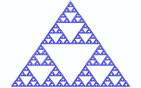
With repeated replacement an straight line segment --- is replaced by, for instance - ^- , or ^, or |^---| a meander. This way ‘twists’ are originating, turning curves, curves baptised with the name of their discoverers, like Levy, Minkovsky, Koch, etc.[45] In the latter there is an analogy with a coastal line; it may be helpful to determine the length of a coastal line and of other whimsical contours.

With repeated transformation (displacement, turning, disfiguring, including diminishing ) figures originate resembling leaves, or branches with leaves. Applying a large number of such appropriately chosen transformations may generate images of non-existing forests, non-existing landscapes with mountains and fjords and even of a human face.

Even ‘fractalising’ an image of a realistic object can be done: that means to say to determine for a sufficient number of transformation formulae each time the 6 parameters in such a way, that they will render that image with great precision.

Further development of this technique is of importance for transmission of images; since these are already determined by a small set of numbers.

In the case of repeated, iterated, application of a formula like z = 2 + C, (where z and C are so-called ‘complex numbers’, that can be represented by a point {x, y} respectively {A, B} in the complex plane, thus allowing calculation of a new point z as the sum of (the old) z squared and the constant C) results in helixes; shrinking or expanding, depending on the initial value of z.

For certain initial values of z border-line cases originate. That is causing then ‘curves’ with a bizarre shape: a JULIA set.

Sometimes it is a connected curve, sometimes the curve consists out of loose, non-connected parts, depending on the value of C.

A set of points C (A,B) establishes the MANDELBROT set. If the computer is ordered to make a drawing of all points C that might deliver a connected JULIA set, another interesting figure is emerging displaying surprisingly fractal character as well.

Whilst zooming in on parts of that figure one discovers complex and fascinating partial structures where in the details de key motifs materialise again and again. Compared to the other fractals discussed here the MANDELBROT fractal is of a higher order.[46]

24.21 Differentiation

From the difference of two evenly succeeding values in a sequence in space or time one can derive the change at a given moment or position. Also, these derived differences can be put into a sequence. If all ‘holes’ between two contiguous values in a sequence are filled (Cauchy-sequence; for instance the sequence of values of a continuous function y), one does not speak any longer of a ‘difference’, Greek capital delta (Δ), (for this has reached its limit to zero), but of a ‘differential’ (d). If the difference in value dy that has approximated zero is divided by the distance in space or time dx between both values that has also approximated zero a ‘differential quotient’ dy/ dx results.

In the graph of a function this quotient stands for the inclination at a certain place or moment. How flat or how steep a motor road is, is also indicated by the ratio between height and length (in percentages). However, in the case of the derived function both are approaching zero, so that they relate only to one point of a curve, instead of a trajectory. The quotient y’= dy/ dx is positive in climbing, negative in descending (see corresponding figure).

Figure 33 Properties of derived functions

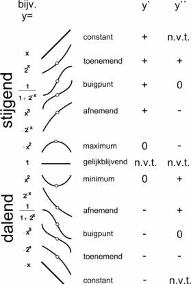
A lot of rules exist in order to formulate for a given function for all values at the same time a derived function. Since Leibniz and Newton these derivations can be proved by and large; but it is not strictly necessary, to know that proof in order to use the rules. Still the question remains, whether the mathematical insight aimed at in an education benefits from absence of proof in the Euclidean tradition. However this insight does not benefit either from applying without comprehension these rules learned by heart. Computer programs like MathCad, Matlab, Mathematica or Maple do apply these rules automatically and unerringly, so that all attention can be concentrated on the external behaviour of the functions and their derivations.

In the previous table one may see that minima, maxima, and turning points can be found by putting the derived function y’= 0 or the derived function of the derived function y’’ = 0, and then calculate the corresponding y. This is especially important for optimising problems. However if one knows of a certain function for instance just that is rises increasingly, one can search contrariwise for a formula for y for which y’ as well as y’’ is positive. For this reversed way (integration) a body of calculation rules is also available.

24.22 Integration

Imagine, that one determines for a symmetrical ridged roof for the time being the width to cover, for instance b = 10m, the height of the gutters (gh) to left and right gh1 = gh2 = 4; the height of the ridge rh1 = rh2 = 9 and the ridge position rp = 0.5b. Then the slope of the surfaces of the roof is depending on this. In Mathcad the calculation looks as follows:

Width and ridge position of a roof:

b = 10 rp = 0,5b

roof-plane left roof-plane right

gh1 = 4, rh1 = 9 rh2 = 9, gh2 = 4

The roof-slopes are now:

The mathematical formula describing the course of the left half between x = 0 (left gutter) and x = rp (ridge) is h1x, to which is added the height of the gutter. However, the part to the right had a descending slope h2 and therefore a different formula between ridge x = rp to the gutter at the right (x = b). Mathcad can assemble both formulae to one discontinuous function f(x) with an ‘if-statement’: ‘if x < rp, then f(x) = gh1 + gh2, else f(x) = rh + h2(x – rp)’. This is described as follows:

Wall function:

Figure 34 A wall as a function

Summed surface area of the wall from 0 to b:

The integral over the width gives the surface area of the front wall. When one is now also taking into account de depth y, this surface may be integrated one more time over y in order to get the cubic content.

Suppose, that the ridge position with the depth y is varying according to a randomly chosen formula rp(y), then the roof slopes h1(y) and h2(y) also vary in depth y:

The wall function now becomes a building function with two variables f(x,y). In the wall function one should only substitute for the constant np the variable rp(y) and do the same for h1 and h2:

When one substitutes for x and y discrete values from 0 to 10, one can store the values in a 10 x 10 matrix Mx,y = f1(x,y). It can be made visible as follows:

Figure 35 A house as a function

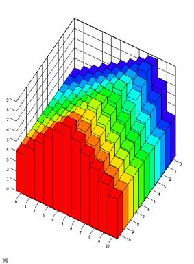
When the values over rows and columns are summed in the matrix one gets a first impression of the content; the double integration of the function f1(x,y) over x and y obviously yields a more exact calculation.

This is particularly convenient, when one is opting for smoothly flowing roof-shapes, for instance:

Figure 36 A house with waved walltops as a function

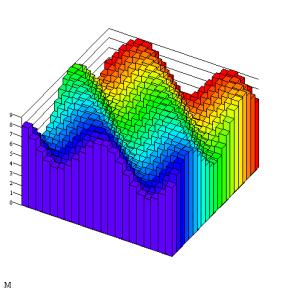
Differential and integral calculus may be understood along the lines of spatial problems; but it is more often applied in the analysis of processes. In that case the differential dx is often indicated by dt and the growth (or shrinkage) on a particular moment in time by:

A well-known example is the acceleration with which a body rolls from a variable slope, like a raindrop from the roof. In architecture calculations for climate control are mainly the ones using differential and integral calculus.

24.23 Differential equations

Population growth offers an example of growth that may grow itself, sometimes constant (k) with the size of the already grown population P(t) itself:

One may verify this even when not knowing a formula for P(t). Such an equation, where an unknown function is occuring together with one or more of its derivations, is called a differential equation. Also in daily parlance primitive differential equations are used: ‘If the population is increasing, the population growth is becoming correspondingly larger’.

Solving a differential equation entails finding formulae for the unknown function (here P(t)). Since the derived function of e^kt is equal to ke^kt,

the derived function of e^kt (ke^kt) is easy to calculate. This is the reason for a preference to express functions as a power of the real number e = 2,718.

However, if one solution for the differential equation is P(t) = e^kt, this does not need to be the only solution. Usually, there is a whole family of solutions. We could have substituted, for instance, Ce^kt; for its derived function is Cke^kt, so that the differential equation also holds in that case. The solutions in the following are by the same token just a few of an infinite number of possible solutions for k = 0.4 (e^k=1,5), for instance:

Figure 37 Powers of e

In order to get to know which formula of this family is the right one, we must know the outcome on any specific moment in time, for instance t=0 (initial value). Supposing that we know that the population was initially 2 people, then we can calculate C from Ce^kt=2. Given that e⁰=1, C=2 applies for each k. In this family of equations C is always the initial value. From this follows the only formula that is correct: P(t)=2e^kt. However, this would mean that if every person would have after 25 years (a generation) 1.5 children on the average (three per couple), there would be after 2000 years (80 generations) 1.579^. 10¹⁴ children.

The hypothesis of constant growth with regard to the population used in our differential equation is not correct. There are limits to the growth put to it by the sustaining power of the environment. This is demonstrated by many other species than Homo sapiens and the real course of the population since 1750 in millions of inhabitants.

Figure 38 Simulated population of The Netherlands

Exponential growth is only valid in the case of relatively small populations. Nearing the boundaries G – established by the size of the habitat – the growth slackens (see also page ). We can add a term to the differential equation realising this:

If P(t) is small compared to G, the term within the brackets approaches 1, so that our original hypothesis remains valid; in the other case the growth becomes 0, or even negative. Logistical curves like the following comply:

The function is a variant of the function mentioned as an example on page . Differential equations are employed to generate from a hypothesis families of functions, allowing selection based on known initial values.

24.24 Systems modelling

Any system has a border; beyond it exogenous variables serve as input for the first functions, they meet within the system. The output of these functions serves on its turn as an input for subsequent functions, sometimes operating in parallel.

The system as a whole delivers in the end an output of tables, images, animations or commands in a process of production.

If a system is modelled on a computer, it is a program that just like a word processing program, awaits input and eventually a command to execute (e.g. the command 'print').

A programming language like Basic, Pascal, C or Java, contains, except mathematical functions, a host of control functions, like 'print(programming language)' , and control statements like 'do…while', 'if …then… else'.

The ‘if…then…’ function, as applied to the ‘wall-function’ on page 35 is a good example for understanding how during the input in a system and during the course of the process – depending on the circumstances – it may be decided which function should operate on the incoming material next and to which following function the result should be passed next as input.

---

[1] Alexander, C. (1977) A pattern language.

[2] Alexander, C. (1964) Notes on the synthesis of form.

[3] Broadbent, G. (1988) Design in architecture: architecture and the human sciences.

[4] Kervel, E (1990) Prisma van de wiskunde 2000, wiskundige begrippen van A tot Z verklaard.

[5] Reinhardt, F., H. Soeder et al. (1977) dtv-Atlas zur Mathematik. Dutch translation: Reinhardt, F. and H. Soeder (1977) Atlas van de wiskunde.

[6] A complete interactive version of the ‘Element’, the ‘Bible’ of geometry, may be found on the internet: http://aleph0.clarku.edu/~djoyce/java/elements/usingApplet.html. It is argued on this site and its links that omitting the Euclidean method in education and exchanging it for a derivation from set theory is detrimental to the logical deduction of conclusions from axioms via propositions to new propositions. The site is interesting by the possibility to change geometrical schemes. This demonstrates the operational character of mathematical propositions and formulae.

[7] Een onderscheid dat door de Griekse wiskundige Proclus werd gemaakt.

[8] Non-Euclidean geometry rejects one or more of these axioms.

[9] Kant, I. (1787) Critik der reinen Vernunft. The programme of this study is summarised particularly clearly in the Preface to this edition. A short introduction to Kant: Schultz, U. (1992) Immanuel Kant.

[10] A well-known publication of CBS is ‘X years in time series’, e.g. Centraal Bureau voor de Statistiek (1989) 1899-1989 negentig jaren statistiek in tijdreeksen.

[11] 'Ho qeos aei geometrei', according to a famous Greek statement.

[12] See Reinhardt, F., H. Soeder et al. (1977) dtv-Atlas zur Mathematik.

[13] Russell, B. (1919) Introduction to mathematical philosophy. Frege, G. (1879) Die Grundlagen der Arithmetik, Ein logisch mathematische Untersuchung über den Begriff der Zahl. English translation: Frege, G. (1968) The foundations of arithmetic: a logico-mathematical enquiry into the concept of number. Dutch translation: Frege, G. (1981) De grondslagen der aritmetica, een logisch-mathematisch onderzoek van het getalbegrip.

[14] Frege, G. (1981) De grondslagen der aritmetica, een logisch-mathematisch onderzoek van het getalbegrip. This problem is described in paragraphs 34 to 54 and proves to be not as easy as it seems.

[15] Stevens, S.S. (1946) On the theory of scales of measurement.

[16] Leede, E. de and J. van Dalen (1996) In en Uit. Statistisch onder-zoek met SPSS for Windows.

[17] Formulation derived from Reinhardt, F., H. Soeder et al. (1977) dtv-Atlas zur Mathematik.

[18] Deelder, J.A. (1991) Euforismen.

[19] An example of a measure-system with equal measures also applies, by the way, to the choice of a resolution.

[20] Hildebrandt, S. and A. Tromba (1985) Mathematics and optimal form. Dutch translation: Hildebrandt, S. and A. Tromba (1989) Architectuur in de natuur: de weg naar optimale vorm.

[21] In case 0!, 0! = 1

[22] This can be done with the formula =FACT(100)/(FACT(25)*FACT(25)*FACT(25)*FACT(25))

[23] Van Tijen (1932) Bergpolderflat (Rotterdam) N.V. Woningbouw, Barbieri, S.U. and L. van Duin (1999) Honderd jaar architectuur in Nederlands, 1901-2000. p. 194

[24] See also Lootsma, F.A. (1999) Multi-criteria decision analysis via ratio and difference judgement.

[25] Kruijtzer, G. (1998) Ruimte en getal.

[26] Aarts, J.M., R.J. Fokkink et al. (2001) Morphic Numbers.

[27] Tummers, L.J.M. and J.M. Tummers-Zuurmond (1997) Het land in de stad. De stedebouw van de grote agglomeratie.

[28] Berger, M. (1987) Geometry II; Berger, M. (1987) Geometry I; Wells, D.G. and J. Sharp (1991) The Penguin dictionary of curious and interesting geometry; Aarts, J.M. (2000) Meetkunde. Dutch translation: Wells, D.G. and J. Sharp (1993) Woordenboek van merkwaardige en interessante meetkunde.

[29] Euclides (310 BC) The Elements (http://aleph0.clarku.edu/~djoyce/java/elements/usingApplet.html)

[30] With a 'network' usually a directed network is implied.

[31] Amongst others, used in programmes like Route Planner, to calculate the shortest path from A to B.

[32] For instance: in order to calculate the time required to realise a building or site.

[33] This form of representation is known as an AON-network: Activity On Node.

Initially only AOA-networks were used with the activities on the arrows (Activity On Arrow). In that case the flow on the arrows represent the temporal duration.

[34] This Latin capital is properly chosen, in view of its form-equivalence with the stream that ‘comes out’ of an urn.

[35] This Greek capital is properly chosen, in view of its form-equivalence with the urn, proverbial in statistical textbooks, turned upside-down and producing arbitrarily red and white marbles.

[36] s := √ ( (S x2 - S x S x / n ) / n )

[37] Convention used: names of unknown variables in capital letters, names of known ones in under-case. In multiplication known precedes unknown, so: a * X

[38] Further reading: Hillier, F.S. and G.J. Lieberman (2001) Introduction to operations research.

[39] X is a column vector, XT the same sequence as a row vector

[40] Horssen, W.T. van and A.H.P. van der Burgh (1985) Inleiding Matrixrekening en Lineaire Optimalisering. describe in which cases that is possible.

[41] For instance in Excel A^-1 is calculated by the function {=MINVERSE(A2:D5)} and x by {=MMULT(F2:I5;K2:K5)} if you indicate a field of 4 x 4, call the function, select the necessary inputfields A^-1 and b and close with ctrl-shift.

[42] A more elaborate introduction in matrix calculation in: Lay, D.C. (2000) Linear algebra and its applications.

[43] The algorithm for stage 1 is with a small addition equal to the one of stage 2.

[44] In the reverse, however, an outcome may be produced by different values of the input.

[45] See http://library.thinkquest.org/26242/Full/index.html

[46] [Mandelbrot, 1983 #759]