1 Water

4.1 Water balance.................................................................................................................. 2

4.1.1 Evaporation and precipitation............................................................................................ 2

4.1.2 Runoff............................................................................................................................ 3

4.1.3 References to Water balance........................................................................................... 4

4.2 River drainage................................................................................................................... 6

4.2.1 River morphology............................................................................................................. 6

4.2.2 Q by measurement........................................................................................................ 11

4.2.3 Q on different water heights in the same profile................................................................. 11

4.2.4 Calculating Q with rounghness........................................................................................ 11

4.2.5 Using drainage data....................................................................................................... 14

4.2.6 Probability of extreme discharges................................................................................... 17

4.2.7 Level and discharge regulators........................................................................................ 19

4.2.8 References to river drainage............................................................................................ 20

4.3 Water reservoirs.......................................................................................................... 22

4.3.1 Terminology.................................................................................................................. 22

4.3.2 Water delivery............................................................................................................... 23

4.3.3 Capacity calculation...................................................................................................... 23

4.3.4 Avoiding floodings by reservoirs....................................................................................... 24

4.3.5 Water management and hygiene..................................................................................... 25

4.3.6 Maps concerning local water management....................................................................... 26

4.3.7 References to Water reservoirs....................................................................................... 27

4.4 Polders............................................................................................................................. 28

4.4.1 Need of drainage and flood control................................................................................... 28

4.4.2 Artificial drainage........................................................................................................... 29

4.4.3 Polders......................................................................................................................... 31

4.4.4 Drainage and use.......................................................................................................... 32

4.4.5 Weirs, sluices and locks................................................................................................ 33

4.4.6 Coastal protection......................................................................................................... 35

4.4.7 References to Polders.................................................................................................... 36

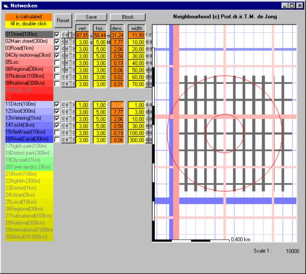
4.5 Networks and crossings.............................................................................................. 37

4.5.1 Networks...................................................................................................................... 37

4.5.2 Crossings..................................................................................................................... 38

4.5.3 Bridges......................................................................................................................... 40

4.5.4 Harbours P.M................................................................................................................ 42

4.5.5 References to Networks and crossings............................................................................ 42

The surface of the Earth is ample half a billion km² and there is 1.39 billion km³ water. So, if water was equally dispersed the Earth would be fully covered by a 2.7km deep ocean (Fig. 1). The 48m upper layer would be ice. However, 29% is land. It contains 3% of all existing water, but 2/3 is frozen.

If all ice would melt by gobal warming sea level would raise 66m.

1000 km3	salt	fresh	total	m3/m2	mm
atmosphere		12,9	12,9	0,025	25
sea	1 338 000		1 338 000	2 624	2 624 021
land, from which	12 957	35 004	47 960	94	94 057
snow and ice		24 364	24 364	48	47 782
subterranean	12 870	10 530	23 400	46	45 891
lakes	85,4	91	176,4	0,346	346
soil moisture		16,5	16,5	0,032	32
swamps		2,1	2,1	0,004	4
life	1,1		1,1	0,002	2
total	1 350 957	35 004	1 385 960	2 718	2 718 079

Fig. 1 Total amount of water on Earth

Fortunately the sun still adds snow to the poles.

1.1 Water balance

1.1.1 Evaporation and precipitation

You can evaporate 1m³ water by 2.26GJ, 2.26GWs, 630kWh or 72Wa (say 72 m³ natural gas). The Earth’s surface receives 81 PW from sun. So the sun could evaporate 1.1 million km³ per year.

Actually less then half is evaporated in unsaturated air only (Fig. 2). It falls down discharging its solar heat in the same time as soon as the air becomes saturated in cooler areas by condensation (precipitation). That is nearly 1m³/m² or 1m and more precise 957mm (Fig. 2).

	evaporation	precipitation	runoff	evaporation	precipitation	runoff
	1000 km3/a			mm/a
sea	419	382		1157	1055
land	69	106	37	467	717	250
total	488	488		957	957

Fig. 2 Yearly gobal evaporation, precipitation and runoff

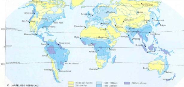
Areas like deserts receive less then 200mm, areas like tropical rain forests more then 2 000mm average per year (Fig. 3).

Wolters-Noordhof (2001) page 181

Fig. 3 Global distribution of precipitation

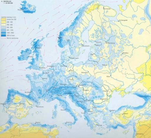
Europe has the same extremes (Fig. 4).

Wolters-Noordhof (2001) page 61

Fig. 4 European distribution of precipitation

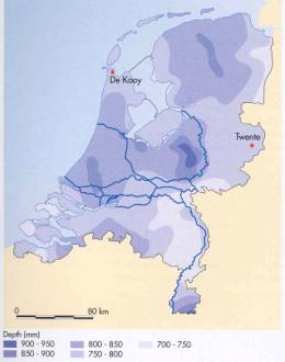
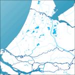
The Netherlands receive from 700mm in East Brabant until 900mm in central Veluwe (Fig. 5), but there have been years of 400mm and 1200mm.


Huisman, Cramer et al. (1998) page 18	Wolters-Noordhof (2001) page 53
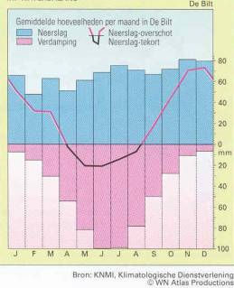
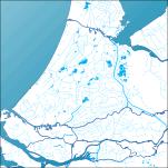
Fig. 5 Distribution of precipitation in The Netherlands	Fig. 6 Precipitation minus evaporation in The Netherlands

1.1.2 Runoff

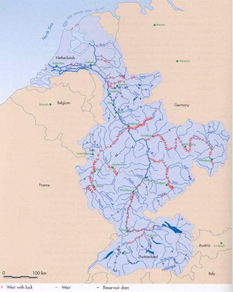
When precipitation exceeds evaporation as soon as lakes and subterranean aquifers have been filled up water runs off subterranean or along brooks and rivers (Fig. 8 and Fig. 9).

Harrison and Harrison (2001)

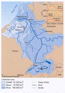
Fig. 7 European river system

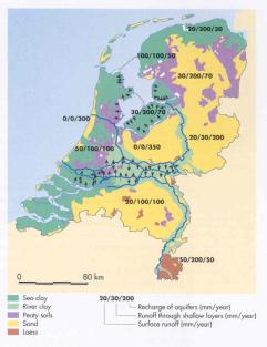
The Netherlands receive runoff from catchment areas of rivers Rhine (entering The Netherlands in Lobith), Meuse and Scheldt (Fig. 7).


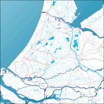
Huisman, Cramer et al. (1998) page 21	Huisman, Cramer et al. (1998) page 13
Fig. 8 Major soil types and average annual runoff in The Netherlands	Fig. 9 Received runoff in The Netherlands

The river Rhine has a catchment area of 180 000km² characterised by 1 775mm precipitation minus 1 392mm evaporation average per year in that area until Lobith. So, 383mm, 69km³/year or at average 2000m³/sec water runs off and comes in at Lobith. Snow and ice in mountains level out season fluctuations of rivers storing precitipation in winter, releasing it in summer. Nevertheless, in February at its normal annual maximum it is 8km³ or 3000m³/sec causing water level 10m NAP at Lobith. But in 1995 17m NAP and 13 000m³/sec is measured at Lobith.

Jong (1995) collected weeks of frontpage news about floodings retrievable in the Chair library. Evacuation of 50 000 inhabitants was ordered by Royal Commissioner of Gelderland Terlouw when floodings threatened Betuwe area behind Lobith in 1995. Afterwards, the threat of floodings caused plans to inundate polders preventively in case of emergency, but a polder of 1km² x 1m = 1 000 000m³ would have stored water for 77 seconds only. So, retention in Rhine basin have to increase, bottoms deepened or dikes along rivers have to be heightened. But which height is enough?

1.1.3 References to Water balance

Harrison, H. M. and N. Harrison (2001) Schiereiland Europa. De hooggelegen gebieden (Berlijn) Reschke & Steffens.

Huisman, P., W. Cramer, et al., Eds. (1998) Water in the Netherlands NHV-special (Delft) NHV, Netherlands Hydrological Society NUGI 672 ISBN 90-803565-2-2 URL Euro 20.

Jong, T. M. d. (1995) Krantenknipsels watersnoodramp 1995 (Rotterdam) NRC.

Wolters-Noordhof, Ed. (2001) De Grote Bosatlas 2002/2003 Tweeënvijfstigste editie + CD-Rom (Groningen) WN Atlas Productions ISBN 90-01-12100-4.

1.2 River drainage

The morphology of a river system and its discharge quantity Q depends on human impact, the proportion of subterranian and surface runoff (Fig. 8), the character and load of transported eroded material and the directions, velocities and quantities caused by slopes in the catchment area.

1.2.1 River morphology

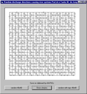
Fig. 10 shows a landscape with 24 x 24 squares (sloped mountain areas or polders) with 4 possible drainage directions, producing converging trucated river systems. Computer programme Jong (2003) ‘river(drainage.exe)’ (see www.bk.tudelf.nl/urbanism/team publications 2003), made from the ‘random walk’ example of Leopold and Wolman cited by Zonneveld (1981), arouses such random landscapes producing river systems. The image is built up in columns from upper left to down below. The programme prevents convergent arrows and smallest circuits by changing lowest arrow 90^o into right or downward if they occur. So, the runoff tends towards ‘South East’ as if the landscape has a main slope. 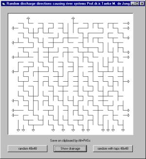Watersheds become visible separating catchment areas. Why do they concentrate into separate basins and converge into main streams? Draw them and calculate the discharge Q for some outputs taking European precipitation and evaporation values into account. Suppose surfaces and altitudes, draw the altitude lines and estimate velocities.


	Zonneveld (1981)
Fig. 10 Directions of drainage in a landscape	Fig. 11 Surface streams caused by Fig. 10

You can divide a river system in different truncation orders from source to output. Fig. 12 shows four methods. Strahler (above right) concerns small source brooks without tributaries above as first order. Streams collecting water form first order are second order rivers and so on. Try to divide Fig. 11 in such orders[a].


Zonneveld (1981) page 179	After Zonneveld (1981) page 183
Fig. 12 Four methods to distinguish ‘orders’	Fig. 13 Average number and length of orders in ‘random walk rivers’

Leopold and Wolman calculated random walk rivers have 4.4 upstream branchings of lower Strahler order at average. In practice it varies between 2 and 5. This ‘bifurcation ratio’ plays a rôle in traffic as well, though street patterns and artificial drainage systems in flat lands are not like a tree but like a lattice (compare Alexander (1966))[1]. If there are 20km streets per km², you can best raise some 7km of them into the order of neighbourhood roads and transform 2km into district ways. So, the optimal proportion between the density of ways and sideways in a lattice seems to be approximately a factor three according to Nes and Zijpp (2000).

Suppose a metropolis of 30km radius has 60 x 60 = 3600km² surface with 2km/km² district ways processing 1000 motor vehicles per hour. There should be 7200km district ways in a grid of average 1x1km. To calculate density from the grid mesh bordered by 4km district roads, you have to count them half because they serve adjacent meshes as well. Many of them would be overloaded by through traffic when you would not raise 1/3 of them into city highways (2400km in a grid of 3x3km, 0.67km/km²) with a capacity of 3000 mv/h and less exits. However, on their turn they would be overloaded. So, this argument produces a semi logaritmic range of orders (Fig. 14).

	km nominal mesh	km/metropolis	km/km² inclusive density	exclusive	mv/h
district roads	1	72000	2,00	1,33	1000
city highways	3	24000	0,67	0,47	3000
local highways	10	7200	0,20	0,13	10000
regional highways	30	2400	0,07	0,05	30000
national highways	100	720	0,02	0,02	100000
and so on			nearly 3.00	2.00	total

Fig. 14 Theoretical orders of urban traffic infrastructure

The total density of ways is 2km/km². One third of them we have transformed into highways of several orders. So, the density of ways includes the highways. Exclusing highways, there are 1.33km/km² small district ways left. If we would like to reduce the amount of exits of local highways to save velocity, we have to disconnect district ways into dead ends. If we like to connect them mutually with extra parallel service roads along side the city highway we need the inclusive density at least.

If we try to draw a system of highways in a square of 60x60km (Fig. 15) we firstly draw a grid of 10x10km. There are 14 local highways of 60km, but 6 of them we transform into a higher order. So, their exclusive density is 8x60/3600=0.13 indeed (Fig. 14). However, we can not fill 10km space between local highways with 3.3 city highways. So we choose 3 highways lowering the inclusive density from 0.67 into 0.60km/km2. This causes a raise of exclusive district way density from 1.33 into 1.40, but on this scale we can not draw them anyhow.



Fig. 15 Orders of dry and wet connections in a lattice

For wet connections the same applies when we call city highways races, local highways brooks and regional highways rivers. The bifurcation ratio of brooks before meeting a river within these regular latices seems to be 20 (Fig. 16 left). However, 4 boundary sections could be used as a mirror axis (dash dotted lines) subsequently counting half. The same density could be reached with a bifurcation ratio 2 and 5 orders (Fig. 16 right).


	Feather like	Tree like
density	29 sections	29 sections
bifurcation ratio	18	2
number of ‘orders’	2	5

Fig. 16 Feather and tree -like connection patterns

In the squares of Fig. 15 tree like connection patterns seem to require a little higher density and consequenly higher costs when restricted to bifurcation ratio 2.[b] If somebody can design a lower density within this boundary conditions I will publish it next time. On the other hand, tree like opening up every point of the area makes many variants and diversity of locations possible when you have more space to lay out (Fig. 17).


	Feather like	Tree like
density	96 sections	98 sections
bifurcation ratio	18	2
number of ‘orders’	2	6 or 9

Fig. 17 Feather and tree like connection patterns opening up a square

Perhaps opening up a 9 x 9 square in a tree-like way with bifurcation ratio 3 could reach the same or even lower densities and consequently lower costs. Try it. Does it result in less nodes and longer sections? The number and characteristics of nodes and the length of sections are important for spatial quality. Which rôle does the length of individual sections L play instead of total length per order in Fig. 13?

The average length L of a random walk river section is related to its catchment area A by L(A)=A^0.64. If length L is given the inverse produces the catchment area, A(L)=L^1.563 (Fig. 18 and Fig. 19).



Fig. 18 Catchment area related to the length of a river section	Fig. 19 Logaritmic representation of Fig. 18

Check Fig. 11 by counting the corresponding squares in Fig. 10 of a specified order and its length. Compare your measurements with Fig. 19 and Fig. 13.

The sections of a river have different morphologies dependent on the coarse-grainedness of transported material and the character of its banks Fig. 20. Near glaciers rough material is laid down in talus. So the water takes diverse and changing courses. Lower sections still bear rough material wearing out the outside parts of a bend into meanders, because rough material laid down there in the same time becomes a water barrier until heavy showers force a break through Fig. 21 and Fig. 22.


From Allan cited by Zonneveld (1981) page 148	From Hoppe cited by Zonneveld (1981) page 149
Fig. 20 Forms of deposit	Fig. 21 Move of Rhine near Neuss from Roman times (a) via Middle Ages (b) until recently

In low lands finer deposits raise the bed in calm periods forcing water to wear away easier courses producing a twining river landscape with temporary islands.


Zonneveld (1981) page 143	Zonneveld (1981) page 144
Fig. 22 Meandering river with historical deposits	Fig. 23 Twining river

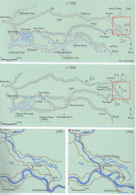
The Rhine area behind Lobith is an example of both processes (Fig. 24).

From Lobith Rhine distributes water via Waal, Lower Rhine and IJssel in historically changing proportions.

Huisman, Cramer et al. (1998) page 38

Fig. 24 Historical distribution of Rhine water from Lobith


Escher 1948 cited by Zonneveld (1981) page 160	Zonneveld (1981)page 161
Fig. 25 Delta development with river (R), top-sets (d) and fore-sets (D)	Fig. 26 Mississippi delta

1.2.2 Q by measurement

The velocity v of water can be measured on different vertical lines h with mutual distance b in a cross section of a river (Fig. 27). You can multiply v x b x h and summon the outcomes in cross section A to get Q = S(v*b*h).

Akker and Boomgaard (2001)

Fig. 27 Profile of a river

For example: asked the river drainage Q (Fig. 29), given h_i, b_i and v_i from profile subdivisions (Fig. 28).


		height h	width b coordinate B	velocity v

Fig. 28 Data from profile


profile subdivisions	drainage per subdivision	velocity	surface	drainage

Fig. 29 Drainage (profile subdivisions and velocities)

1.2.3 Q on different water heights in the same profile

H varies, but you can measure it easily. Then you can calculate drainage Q(H) by a formula characteristic for the profile concerned. However, periods of high drainage Q or regular floodings in winter change profile and formula. Comparing measurements like in paragraph 1.2.2 on different water heights you find a curve often looking like a parabola, approached by Q = a*H^b or H=(Q/a)^1/b (Fig. 30). Parameters ‘a’ and ‘b’ characterise the profile.


	Akker and Boomgaard (2001)}.}.
Fig. 30 ‘Measurements’ M_i and Q(a,B,H) = aH^B or the inverse H(a,B,Q)=* (Q/a)^1/B to get H on the y-axis	Fig. 31 Change of boundary condition downstream; a ‘drowning’ waterfall

Measurements deviate from the formula because velocity varies. When measuremens can not be simulated by a smooth curve, probably boundary conditions downstream change by high water levels. Then you have to make two graphs, one until the point of change, one for the higher values. When for example a waterfall downstream suddenly ‘drowns’ at increasing water levels (Fig. 31) the slope of the curve can change by sudden increase of velocity. When Q=0 at H₀ ¹ 0, for instance when we want to express H₀ related to a reverence surface like NAP, we need a correction like Q = a(H-H₀)^b.

You can find constants a and b by the least squares method provided by Excel using graphs. Put measurements of height and drainage calculated according to Fig. 30 in two columns. Make a point graph and select it. Choose ‘add trend’ in ‘graph’ from the main Excel window above,


choose power,	click both lowest,	click axis,	choose logarithmic,

and you produce graphs like Fig. 32 and Fig. 33 with power regression line and formula.

With R² near to 1 you have a reliable formula. In Fig. 32 we used ‘measurements’ of Fig. 30 putting the independently variable measurements on the x-axis this time to find a=0.0003 and b=8.7398.



Fig. 32 ‘Measurements’ M_i and Q(a,b,H) = a*H^b	Fig. 33 Logarithmic representation of Fig. 32

The logarithmic representation log Q = log a + b log (H-H₀) produces a straight line easy to extrapolate to other heights and drainages. But be careful, there could be jumps in velocity by downstream events. If you have made graphs before and after the jump because measuremens could not be simulated by a smooth curve, each interval in Fig. 33 has different slopes representing different behaviour.

1.2.4 Calculating Q with rounghness

Just like wind, water slows down by roughness of the bed. The cross length of roughness in a wet profile P (Natte Omtrek) is calculated by summing hypothenuses of triangles according to Pythagoras characterised by the square root of (b_i)²+(h_i‑h_i‑1)² (see Fig. 27 and Fig. 35).

Considering the profile as a function H=f(x) we can read the waterlevel H from accompanying left border x₁=l and right border x₂=r as values from f(x) (Fig. 34). The cross length of roughness P (Natte Omtrek) and the surface of the wet cross section A are both calculated as a function of H (Fig. 35).

P

H

A

Cross length by Pythagoras:

Surface wet cross section:

Fig. 34 Profile as a function

Fig. 35 Calculating wet cross section A and cross length of roughness P (NatteOmtrek)

When we divide the surface of the wet cross section A of a stream by this cross length of roughness P we get a measure indicating what part of the flowing water is hindered by roughness called ‘hydrolic radius’ R = A/P in metres.

Method Chézy

The average velocity of water v = Q/A in m/sec is dependent on this radius R, the roughness C it meets, and the slope of the river as drop of waterline s, in short v(C,R,s).

According to Chézy v(C,R,s)=CÖRs m/sec, and Q = Av = ACÖRs m³/sec. Calculating C is the problem.

Method Strickler-Manning

Instead of v=CÖRs, Strickler-Manning used with roughness n token from Fig. 36.

_{Characteristics of bottom and slopes}	_n
	_from	_until
_Concrete	_0.010	_0.013
_{Gravel bed}	_0.020	_0.030
_{Natural streams:}
_{Well maintained, straight}	_0.025	_0.030
_{Well maintained, winding}	_0.035	_0.040
_{Winding with vegetation}	_0.040	_0.050
_{Stones and vegetation}	_0.050	_0.060
_{River forelands:}
_Meadow	_0.035
_Agriculture	_0.040
_Shrubs	_0.050
_{Tight shrubs}	_0.070
_{Tight forest}	_0.100
Akker and Boomgaard (2001)
Fig. 36 Indication of roughness values n according to Strickler-Manning

Method Stevens

Instead of v=CÖRs Stevens used v=cÖR considering Chézy’s CÖs as a constant c to be calculated from local measurements. So, Q = Av = cAÖR m³/sec and c is calcuated by c=(AÖR)/Q. When we measure H and Q several times (H₁, H₂ …H_k and Q₁, Q₂ … Q_k), we can show different values of A(H)ÖR(H) resulting from Fig. 35 as a straight line in a graph (Fig. 37). We can add the corresponding values of Q we found earlier in the same graph reated to A(H)ÖR(H). When we read today on our inspection walk a new water level H1 on the sounding rod of the profile concerned we can interpolate H1 between earlier measurements of H and read horizontally an estimated Q1 between the earlier corresponding values of Q to read Q from graph.

Fig. 37 Graph used according to Stevens with ‘measurements’ of Fig. 32

However, from these ‘measurements’ c appears to be not very constant, but the graph remains a practical way to estimate Q from H.

1.2.5 Using drainage data

Once you collected drainage data throughout a year you can put them in a hydrograph (afvoer-verlooplijn).

Akker and Boomgaard (2001)}.}.

Fig. 38 River with continuous base discharge

Fig. 39 River with periodical base discharge

Fig. 38 shows peaks caused by periods of much precipitation and fast discharge. Fig. 39 shows the behaviour of a season bound river, periodically dry.

A duration line (Fig. 40) shows frequency of discharges arranged from minimum to maximum. The x‑axis shows how long river discharges are less then indicated on y-axis. The river characterised in Fig. 40 never falls dry: 0% of time it has less discharge then indicated on the y-axis left, but the maximum discharge is indicated right: the whole period concerned it was less then that.

A duration line is not a probability curve to estimate discharge on a certain day. After all, river discharges on subsequent days are not independent, but strongly related in periods like seasons. Cumulated periodes of low discharge may indicate measures to prevent shortages in use of water. Cumulated periods of highest (peak) discharges determine measures concerning maintenance, prevention of risks and design. The longer the included time series, the more useful they are. Often they are not long enough to determine a design frequency considering the life span of civil works.


Akker and Boomgaard (2001)	Akker and Boomgaard (2001)
Fig. 40 Duration line	Fig. 41 Dataset with peak discharges

1.2.6 Probability of extreme discharges

Drainage hydrology knows two data sets characterising peak discharges; annual maximum series indicating maxima only and partial duration series indicating peaks exceeding a reference level like the top of summer dikes. Fig. 41 shows an example of both. To make discharges statistically independent we use separate ‘river years’. P₁ - P₄ are an annual maximum series of 4 river years. To make a partial duration series we need P₁', P₃' and P₄' as well. The lower the reference level, the more peaks we take into consideration.

The peak discharge Q_T exceeded once in average T years (‘return period’) is called ‘T-years discharge’. Even if Q exceeds Q_T once in average 10 years (T=10year) it can happen 2 years in succession. There are large fluctuations round the average. Extreme values vary more per year then per 10 year. For T>10 we can use extreme values of highest and lowest values known from the past. If there are no discharge data you can ask older people or read markings of historical high water level former inhabitants left behind. However they are not useful if river morphology (profile) and subsequently Q(H) has changed by nature, artificial normalisation or raising dikes.

The probability of extreme values is called ‘extreme value distribution’. It is described in different ways, for instance like Gumbel type I for maxima, Weibull type III for minima, Log-Gumbel, Pearson or Log-Pearson type III distribution.

In 1941 Gumbel described an extreme value distribution, successful in hydrological applications since then. The Gumbel I distribution is often used for maximum discharges. It supposes independent observations of extreme values X₁, X₂, X₃...X_n (for example successive year maxima) to be exponentially distributed. Then P’, the cumulative probability discharge will be equal to or smaller then earlier observations learned (Q£X) is approximated by P’ = exp(-exp(-y)) and the reverse y = -ln(-ln(P’)). The complementary probability P = 1 ‑ P’ discharge Q will exceed an observation (Q>X) is 1/T and the reverse P’ = 1 – P = 1 – 1/T. So, the ‘reduced variable’ y = -ln(-ln(1 – 1/T)).

When we arrange the measurements from maximum m=1 until minimum m=N (the number of years we were measuring), return period T = (N+1)/m (‘plotting position’) and P = m/(N+1).

To resume: , . So, we can make a graph expressing P in y.

But we can also express T in y and make a graph (Fig. 42).

Fig. 42 shows return period once a year (T) has probability 1 (P), once in two years has probability 0.5 or 50%. Both are expressed in y. To see once in 1000 years we should represent the vertical axis logaritmically (Fig. 43). The Gumbel I distribution becomes a straight line when we stretch out T and P properly around their common value 1. Then T and P look proportional to y. In that case we can put them on the horizontal axis alongside y to get so called ‘Gumbel paper’ (Fig. 44). The vertical axis now is free to give water level H a place. When we know how many times every observed water level occurred last years, we can calculate the return time T, put the observation on Gumbel paper and read immediately the probability P of that observation without calculating reduced variate y. Many observa-tions give a cloud of points. We can draw a straight line though that cloud and estimate which water level could occur in 1000 years or the reverse formulate a risk and read the desired height of dikes!



Fig. 42 T(y) and P(y)	Fig. 43 Fig. 42 Logaritmically	Fig. 44 Gumbel I paper

The horizontal axis of Fig. 44 is ‘Gumbel distributed’. You can distribute the vertical axis logarithmically if there is much sprawl in the cloud of observations. Some observations could deviate too much to be reliable. They could be observed wrongly, calculated, put on paper or even emerge by copying.

Akker and Boomgaard (2001)}.}.

Fig. 45 Estimating an extreme value graph missing data

To analyse extreme minimal discharges you can use ‘log – Gumbel III distribution’ with plotting position T=(N+0.5)/(m-0.25) so, P=(m-0.25)/(N+0.5).

When you have no properly measured discharge data one should rely on information about water levels in the past. For one point in the graph you can assume ‘bank full level’ once in 1.5 year (Fig. 45). This corresponds to usual height of dikes or raisings along the banks. A next point in the graph could be obtained from markings by the inhabitants (for example the highest level in the past 20 years).

1.2.7 Level and discharge regulators

Ankum (2003) page 156

Fig. 46 Level regulator with level as target

Ankum (2003) page 156

Fig. 47 Discharge regulator with discharge as target

Ankum (2003) page 167

Fig. 48 ‘Manners’ of regulation

The fixed regulators are called weirs (stuwen), manual or automatic regulators are called gates (schuiven).

1.2.8 References to river drainage

Akker, C. v. d. and M. E. Boomgaard (2001) Hydrologie (Delft) DUT Faculteit Civiele Techniek en Geowetenschappen.

Alexander, C. (1966) A city is not a tree (London) [s.n.].

Ankum, P. v. (2003) Polders en Hoogwaterbeheer. Polders, Drainage and Flood Control (Delft) Delft University of Technology, Fac. Civiele Techniek en Geowetenschappen, Sectie Land- en Waterbeheer: 310.

Huisman, P., W. Cramer, et al., Eds. (1998) Water in the Netherlands NHV-special (Delft) NHV, Netherlands Hydrological Society NUGI 672 ISBN 90-803565-2-2 URL Euro 20.

Jong, T. M. d. (2003) Riverdrainage.exe (Zoetermeer) MESO.

Nes, R. v. and N. J. v. d. Zijpp (2000) Scale-factor 3 for hierarchical road networks: a natural phenomenon? (Delft) Trail Research School Delft University of Technology.

Zonneveld, J. I. S. (1981) Vormen in het Landschap. Hoofdlijnen van de geomorfologie (Utrecht / Antwerpen) Uitgeverij Het Spectrum ISBN 90-274-6209-7.

1.3 Water reservoirs

Snow and ice in mountains are most important forms of water storage. They level out season fluctuations of rivers like Rhine storing precitipation in winter, releasing it in summer when we need it most. At lower scale water reservoirs buffer fluctuations in runoff for water supply in dry periods, provide 23% of world electricity production and avoid downstream floodings (retention). Retention in Rhine Basin has great impact on runoff reaching Lobith (Fig. 49).

Huisman, Cramer et al. (1998)

Fig. 49 Retention in Rhine basin

Within the Netherlands water is stored in shallow reservoirs. Afsluitdijk and Detawerken created large reservoirs for watermanagement in The Netherlands. They are primarily meant for safety, but serve more purposes. For example, the Northern Delta basin serves fresh water supply and stop the inward push of salt water. Rhine water now can be used for water demand around IJsselmeer and makes river IJssel navigable. IJsselmeer stores remaider of precipitation in winter to meet the demand of agriculture in summer. Summer and winter water level in the IJsselmeer is regulated by weirs in Afsluitdijk. Outlet waterways around polders (boezem) serve as reservoirs as well. Polders themselves have regulated water levels (polderpeil) as negative reservoirs with inlets and outlets on boezem waters.

1.3.1 Terminology

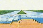
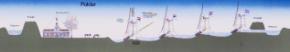
A water reservoir has ‘useful storage’ (nuttige berging) S and ‘dead storage’ (dode berging) below discharge opening (Fig. 50).

The height and width of a possible emergency overflow determines maximum capacity. Surface A is largest there, so the extra (effective) storage slowing down high upstream discharge avoiding floodings downstream can be substantial, be it not useful for other purposes (Fig. 50).

The storage of original river bed (dotted line in Fig. 50) is hardly part of effective storage, but nearly fully part of artificial useful storage.

Akker and Boomgaard (2001)

Fig. 50 Terminology of reservoirs (example with barrage).

When surface A varies with height h storage S is not proportional to height. By measuring surfaces on different heights A(h) you get an area-elevation curve (Fig. 51). The storage on any height S(h) (capacity curve) is the sum of these layers or integral .

Akker and Boomgaard (2001)

Fig. 51 A(h) and S(h)

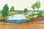
Fig. 51 left below shows dead storage, important to avoid fish mortality, ecological damage and stench. It makes sedimentation possible without loss of useful storage.

1.3.2 Water delivery

The time you can deliver a desired capacity (yield) can vary from days (distribution reservoir with small storage) to years (large storage reservoir), dependent on instream. The maximum yield during a normative dry period is called ‘save yield’. There is always a possibility of dryer periods then normative. So, determining save yield requires a probability approach.

The maximum water delivery equals instream plus accepted decrease of useful storage minus often substantial evaporation and leakage. Increasing fluctuation of instream increases the necessity of useful storage; constant instream would make storage superfluous.

The choice of reservoir capacity depends on both desired delivery capacity and accepted risk of incidental non delivery. Irrigation systems can stand larger risks (for example 20% of time delivery below design capacity) then much more sensible urban water supply systems

1.3.3 Capacity calculation

You can simulate the working of a reservoir (‘operation study’) based on runoff data of daily (small reservoirs), monthly (normal) or yearly (very large reservoirs) intervals in the existing river. Do not restrict to ‘critical periods’ of low runoff. Long term runoff series give a better reliability comparison of different capacities. Fig. 55 shows the cumulative sum of input minus output (inclusive evaporation and leakage). The graph is divided in intervals running from a peak to the next higher peak to start with the first peak. For every interval the difference between the first peak and its lowest level determines the required storage capacity of that interval. The highest value obtained this way is the required reservoir capacity.

Akker and Boomgaard (2001)

Fig. 52 Determining necessary storage capacity

In 1883 Rippl introduced the ‘Rippl diagram’ (Fig. 53) summing input minus evaporation and leakage into an increasing line. The slope is proportional to the net input. Constant water demand is represented by straight lines. You can move them until they touch the ultimate points of the summing curve (A, B and C; in these points the increasing useful storage changes into decrease). Exactly where the straight line behind such a point crosses the curved one the reservoire is full again. The maximum vertical distance between demand line and summing curve FG is the required capacity. The vertical distance between two successive demand lines (BH) is discharged by emergency overfow.


	Akker and Boomgaard (2001)
Fig. 53 Rippl diagram	Fig. 54 Exploitation of a reservoir

If demand is not constant it becomes a curved line, but the analysis remains the same. In that case you can move the demand line vertically only to keep time of supply and demand the same.

A summing curve can be used to determine water delivery at given capacity as well. Then demand lines should be moved to a vertical distance not larger then that given capacity and crossing the summing curve somewhere later otherwise the reservoir will never be filed up again. The slope of the demand lines represents maximum delivery in the period concerned.

Fig. 54 shows the exploitation of a reservoir in a given period starting with a storage S₀ in the beginning of the first year. After some months the content decreases up to 0, but a large input fills the reservoir completely. The arrow has the same length as FG from Fig. 53. From this moment until delivery is larger than input water is discharged by emergency overflow. The vertical distance between input and tota output does not change as long as the reservoir is full. Then a period of decrease and increase follow until the reservoir is full again. Fig. 54 shows an empty reservoir in F because capacity was calculated by the difference of supply and demand in this point.

To keep summing curves manageable for ever increasing large amounts of water in periods long enough to be reliable you can subtract an average discharge. Then the reduced summing curve fluctuates around a horizontal line rising when input is larger then average and descending when smaller.

Before deciding for a capacity often more detailed studies about leakage as a function of water level and evaporation as a function of surface are made related to one or more periods with available data. Computer models can test the usefulness of different strategies.

1.3.4 Avoiding floodings by reservoirs

A reservoir can be used for more purposes at once, but used only to avoid floodings downstream it is called a retention reservoir. To avoid floodings you have to take longer periods of high input then incidental peaks into account. A retention reservoir should be as empty as possible if you expect a high water wave. In that case you open discharge openings as soon as possible before the expected wave comes to increase storage capacity and to postpone emergency overflow as long as possible. Risk = probability x consequence. To estimate the risk a reservoir can not store runoff long enough you need to know probability distributions of daily discharge (Fig. 55 above), regular output as a function of water level in the reservoir, and other factors like consequences of unverifiable overflow.

Akker and Boomgaard (2001)

Fig. 55 Probability distribution daily discharge and exceeding probability

Fig. 55 below shows the accumulated probability distribution. The dotted line shows 10% probability a discharge on vertical axis is exceeded. In practice much smaller probabilities are used, for instance 0.1%. Simply stated it corresponds 0.1 x 365/100 = 0.365 day per year » once per 3 year if you take a day as unbroken period.

1.3.5 Water management and hygiene

Construction of reservoirs has environmental impacts. It requires space at the expense of original functions. Losses can not only be expressed in money. Landscape and nature have emotional or intrisic value as well. Weighting advantages and disadvantages is difficult, the more so because the intended function can not be guaranteed for 100% and side effects can not be predicted. For example the Assuan dam changed Nile delta substantially. Nile transports less slugdge. So, measurements against erosion of coast became necessary. Irrigation alongside Nile increased, but bilharzia disease dispersed in a large area as well.

The storage of water in the lower parts of The Netherlands will require heavy surface claims. The 4^th National Plan of watermanagement policy V&W V&W (1998) (stressing environment), and its last successor ‘Anders omgaan met water’ V&W (2000) (stressing security) mark a change from accent on a clean to a secure environment, just as the 4^th National Plan of environmental policy VROM (2001) compared with its predecessors[2]. Several floodings in The Netherlands and elsewhere in Europe has focused the attention on global warming and watermanagement. The future problems and proposed solutions are summarized in the figures below[3]. Storage is a central item reducing risks of lowlands.

	In Fig. 56 above most left, global warming, in the figure right the ground descend of the western and northern part of the Netherlands are shown. Bottom most left, different scenarios of temperature increase, right of it, the expected increase of precipitation in winter and decilne in summer are shown.
V&W (2000)
Fig. 56 Expected problems	Fig. 57 Strategies: 1 care, 2 store, 3 drain

Water management is recognisable everywhere in the lowlands.

Das (1993)

Fig. 58 Lowlands with spots of recognisable water management

Civil engineering offices are busy with many water management tasks (Fig. 59).


01 Water structuring	02 Saving water	03 Water supply and purificatien	04 Waste water management

05 Urban hydrology	06 Sewerage	07 Re-use of water	08 High tide management

09 Water management	10 Biological management	11 Wetlands	12 Water quality management

13 Bottom clearance	14 Law and organisation	15 Groundwater management	16 Natural purification
Das (1993)
Fig. 59 Water managemant tasks in lowlands

1.3.6 Maps concerning local water management

The Netherlands are covered by maps showing the compartments governing their own watermanagement (Waterschappen), and their drainage areas (Fig. 60 above). Overlays show hydrological measure points (Fig. 60 below left) and the supply of surface water (Fig. 60 below right).


Rijkswaterstaat (1985)

Rijkswaterstaat (1984)	Rijkswaterstaat (1984)
Fig. 60 Hydrological maps of Delft and environment.

On the first map you can find the names of compartments, pumping-stations, windmills, sluices, locks, dams, culverts, water pipes.

1.3.7 References to Water reservoirs

Akker, C. v. d. and M. E. Boomgaard (2001) Hydrologie (Delft) DUT Faculteit Civiele Techniek en Geowetenschappen.

Das, R. (1993) Integraal waterbeheer werken aan water (Deventer) Witteveen + Bosch.

Huisman, P., W. Cramer, et al., Eds. (1998) Water in the Netherlands NHV-special (Delft) NHV, Netherlands Hydrological Society NUGI 672 ISBN 90-803565-2-2 URL Euro 20.

Rijkswaterstaat (1984) Hydrologische waarnemingspunten Rotterdam - Oost 37 (Delft) Meetkundige Dienst.

Rijkswaterstaat (1984) Watervoorziening Rotterdam - Oost 37 (Delft) Meetkundige Dienst.

Rijkswaterstaat (1985) Waterstaatskaart van Nederland Rotterdam - Oost 37 (Delft) Meetkundige Dienst.

V&W, M. v. (1998) Waterkader Vierde Nota waterhuishouding. Verkorte versie (Den Haag) Ministerie V&W.

V&W, M. v. (2000) Anders omgaan met water. Waterbeleid in de 21e eeuw. (Den Haag) Ministerie van Verkeer en Waterstaat.

VROM, M. v. (2001) Een Wereld en een Wil. Werken aan duurzaamheid.Nationaal Milieubeleidsplan 4 - samenvatting (Den Haag) Ministerie van Volkshuisvesting, Ruimtelijke Ordening en Milieubeheer ISBN vrom 010294/h/09-01.

1.4 Polders

1.4.1 Need of drainage and flood control

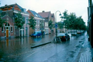
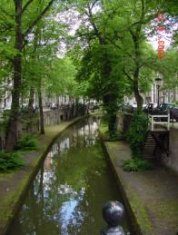
Urban areas need dry crawl spaces to keep unhealthy moist out of the buildings but they need wet foundations as long as they are made of wood. Let us say groundwaterlevel (recognisable from open water in the area) should stay at least 1m below ground level (Fig. 61, Fig. 62).


(Paul van Eijk)
Fig. 61 Flooding of a canal in Delft	Fig. 62 Deep canal in Utrecht

Grasslands may be wetter, dryland crops should be dryer then 1m below terrain (Fig. 63).

Ankum (2003) page 53

Fig. 63 Crop yields for different open water levels

Lowlands with drainage and flood control problems cover nearly 1mln km² all over the world (Fig. 64) and nearly half world population lives there because of water shortage elsewhere (Rijkswaterstaat (1998; Rijkswaterstaat (1998; Rijkswaterstaat (1998)).

x1000 km2	1 crop	2 crops	3 crops	Total
North America	170	210	30	400
Centra America		20	190	210
South America	60	290	1210	1560
Europe	830	50		880
Africa		300	1620	1920
South Asia	10	460	580	1050
North and Central Asia	1650	520	20	2190
South-East Africa			530	530
Australia		310	120	430
				9170
Ankum (2003), page 2
Fig. 64 Area of lowlands with drainage and flood control problems

1.4.2 Artificial drainage

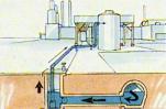
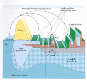
Inhabitated or agricultural areas below high tide river or sea level (polders) have to be drained by one way sluices using sea tides or pumping stations (Fig. 65, Fig. 67), surrounded by belt canals (boezemkanalen), protected by dikes, made accessible for shipping traffic by locks, internally drained by races (tochten), main ditches (weteringen), ditches (sloten), trenches (greppels), and pipe drains.

Ankum (2003), page 78

Fig. 65 Pumping stations in The Netherlands

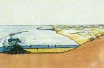
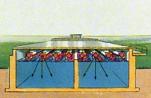
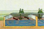
Pumping in polders with different altitudes can be done at once from the deepest part using gravity or in compartiments separated by dikes and weirs saving potential energy (Fig. 67).



Huisman, Cramer et al. (1998) page 36 ; Veer (?)	Ankum (2003), page 76 and 55
Fig. 66 Lowland system	Fig. 67 Drainage by one to three pumping stations, in earlier times by a ‘row of windmills’ (‘molengang’)

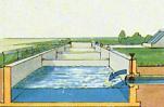
Water is drained by one way sluices (Fig. 68) at low tide or pumped up via belts (boezems) into the river or the sea.


Ankum (2003), page 68 and 38
Fig. 68 The oldest one way sluice found in The Netherlands and its modern principle

Fig. 69 shows the belt system of Delfland.

Ankum (2003) page 62

Fig. 69 The belt (‘boezem’) system of Delfland

One way sluices lose purpose when average sea and river level raise and ground level drops mainly because of the subsidence of peat polders (Fig. 70). Drying peat oxidates and disappears.

Ankum (2003) page 71

Fig. 70 Rising outside water levels and dropping ground levels

1.4.3 Polders

Polders are optimally drained by a regular pattern of ditches (Fig. 71, Fig. 72).


Ankum (2003) page 42 and 82
Fig. 71 Hachiro Gata Polder in Japan	Fig. 72 Wieringermeer polder (Kley 1969)

The necessary distance L between smallest ditches or drain pipes is determined by precitipation q [m/24h], the maximally accepted height h [m] of ground water above drainage basis between drains and by soil characteristics.


Ankum (2003) page 36
Fig. 73 Variables determining distance L between trenches	Fig. 74 Variables determining distance L between drain pipes

Soil is characterised by its permeability k [m/24h].

*Type of soil*	*Permeability k in m/24h*
gravel	>1000
coarse sand with gravel	100	1000
corse sand, frictured clay in new polders	10	100
middle fine sand	1	10
very fine sand	0.2	1
sandy clay	0.1
peat, heavy clay	0.01
un-ripened clay	0.00001

Fig. 75 Typical permeability of soil types

A simple formula is L=2Ö(2Kh/q). If we accept h=0.4m and several times per year precipitation is 0.008m/24h, supposing k=25m/24h the distance L between ditches is 100m. However, the permeability differs per soil layer. To calculate such differences more precise we need the Hooghoudt formula desribed by Ankum (2003) page 35.

1.4.4 Drainage and use

However, plot ditches are used as property boundaries and they determine agricultural and urban practice. Any use has its own requirements for plot division. Systems of plot division have to take dry infrastructure into account, combining different network systems.

Ankum (2003) page 59

Fig. 76 Alternative systems of plot division in polders

We will elaborate that in 1.5

1.4.5 Weirs, sluices and locks

There are many types of water level regulators elaborated by Arends (1994) (Fig. 77, Fig. 78, Fig. 79).


Schotbalkstuw	Schotbalkstuw met wegklapbare aanslagstijl	Naaldstuw	Automatische klepstuw

Dakstuw	Dubbele Stoneyschuif	Wielschuif rechtstreeks ondersteund door jukken	Wielschuif via losse stijlen ondersteund door jukken
Arends (1994)

Fig. 77 Types of weirs


Uitwateringssluis open	Uitwateringssluis closed	Inlaatsluis open	Inlaatsluis closed

Irrigatiesluis	Ontlastsluis closed	Ontlastsluis flooded	Ontlastsluis open

Keersluis	Spuisluis	Inundatiesluis (military)	Damsluis (military)
Arends (1994)

Fig. 78 Types of sluices

To allow accessibility of shipping traffic you need locks at every transition of water level.


Schutsluis

Dubbelkerende schutsluis

Gekoppelde sluis	Sluis met verbrede kolk	Bajonetsluis

Tweelingsluis	Schachtsluis	Driewegsluis
Arends, G.J.(1994) Sluizen en stuwen (Delft) DUP Rijksdienst voor de Monumentenzorg

Fig. 79 Types of locks

Any regulator, culvert, sluice, lock or bridge requires a structure with entrance and exit of water needing space themselves (Fig. 80).

Ankum (2003) page 164

Fig. 80 Samples of the ‘entrance’ and ‘exit’ of a structure

1.4.6 Coastal protection

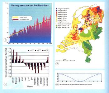
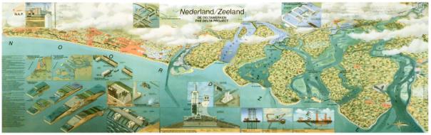
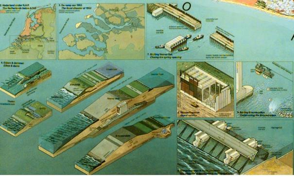
Floodings in 1953 caused the Delta Project, the greatest coastal protection project of The Netherlands, (Fig. 81) showing many modern constructions.

Hettema and Hormeijer (1986)

Fig. 81 Delta project

1.4.7 References to Polders

Arends, G. J. (1994) Sluizen en stuwen. De ontwikkeling van de sluis- en stuwbouw in Nederland tot 1940 (Delft) Delftse Universitaire Pers / Rijksdienst voor de Monumentenzorg ISBN 90-6275-700-6.

Hettema, T. and P. Hormeijer (1986) Nederland/Zeeland (Amsterdam) Euro-Book Productions.

Huisman, P., W. Cramer, et al., Eds. (1998) Water in the Netherlands NHV-special (Delft) NHV, Netherlands Hydrological Society NUGI 672 ISBN 90-803565-2-2 URL Euro 20.

Rijkswaterstaat (1998) "Delta's of the World. 200th anniversary of Rijkswaterstaat" Land + Water 11

Rijkswaterstaat (1998) Summary and Conclusions (SDD '98) International conference at the occasion of 200 year Directorate-General for Public Works and Water Management, Conference (Location) Delft University Press.

Rijkswaterstaat (1998) Sustainable Development of Deltas (SDD '98) Inetrnational conference at the occasion of 200 year Directorate-General for Public Works and Water Management, Conference (Location) Delft University Press.

Veer, K. v. d. (?) Nederland/Waterland (Amsterdam) Eurobook productions.

1.5 Networks and crossings

1.5.1 Networks

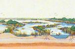
Although natural drainage follows a dendritic pattern, this is crossed by a predominantly orthogonal system of dry channels with similar hierarchical orders. For various reasons, there is a tendency for the artificial drainage of flat areas to be rectangular in shape. Because of this, the following considerations apply to both wet and dry networks. Fig. 82 shows a sequence of relationships between mesh lengthand width.in rectangular meshes with a net density of 2 km per km^2.


	Hildebrandt and Tromba (1989)
Fig. 82 Length (L) and width (W) of the mesh for a given net density of (D=2)	Fig. 83 The formation of right angles

Length and width of squares are 2/d.The same density also occurs in a pattern of roads that go infinitely in one direction every 0.5 km. Thus, when the length and width of the mesh 1/d = 0.5 km, the ratio between length and width is at its limit. In that case, where the net density is 2 km per km²there canbe no ‘crossroads’ any more.

This consideration only applies to an orthogonal system. The most efficient enclosure is made by encircling the enclosed area with a minimum length of road. As is well known, this is the circle, but in a continuous network, this is approximated by a hexagonal system,. This minimal ratio between periphery and area is demonstrated three dimensionally by very many natural phenomena where preference is given to a minimal ratio between area and content[c]. A good example is a cluster of soap bubbles. A cluster of soap bubbles forced into a thin layer produces a two-dimensional variant. The bubbles arrange themselves in polygons with an average of six angles. If one then pulls a thread through them, the nearest bubbles will re-arrange themselves again into an orthogonal pattern (Fig. 52). Urban developments from radial to tangential can also be interpreted against this background. The interlocal connections pull the radial system straight, as it were. The additional demand for straight connections over a distance longer than that between two side roads (called a ‘stretch’ here) introduces rectangularity. Every deflection from the orthogonal system is then less efficient.

This can be clarified by engaging in a thought experiment: Imagine a rectangular framework with hinged corners that is completely filled with marbles. If one re-shapes this framework into an ever narrower parallelogram, then there will be space for fewer and fewer marbles, so, in every case, the rectangular shape proves to be optimal, in this respect[d].

Fig. 84 Styling wet connections, where the density is translated into nominal orthogonal mesh widths.

The density in the pattern of drainage ditches shown on a topographical map, gives one a global picture of the soil types of that area. There are no ditches on sandy soils, whereas a wide mesh of ditches is a characteristic of clay soils and a fine mesh, of peaty soils (for examples, see Fig. 84). For convenience, the breadth of each watercourse is fixed here at 1% of the equilateral mesh width.

This difference is caused mainly by different vertical percolation of water k expressed in metres per twenty-four hours. That percolation is slow in peat and clay (for example 20m/24h at average in the low West Holocene of the Netherlands) and fast in rough sand (350m/24h in the higher East Pleistocene of the Netherlands or sand raised town areas). Density d of lowest order ditches or brooks depends further from once a year maximum precitipation N in metres per twenty-four hours (for example 0.007 m/24h or 0.008m/24h) and the difference between ditch level and ground water level in the area between ditches or brooks h (for example 0.4m). Then, d(k,N,h)=250Ö(2N/kh) km/km² (Fig. 85)

	Peat	Clay	Sand
Percolation k [m/24h]	6	23	280
Precipitation N [m/24h]	0.007	0.007	0.008
Waterlevel between ditches h [m]	0.4	0.4	0.4
Network density d [km/km²]	20	10	3

Fig. 85 Network density caused mainly by soil characteristic of percolation

1.5.2 Crossings

Mutually crossings of waterways seldom separate their courses vertically (Fig. 86) as motorways do (Fig. 87).


Ankum (2003) page 160	Standaard and Elmar (?)
Fig. 86 Crossing of separated waterways	Fig. 87 Crossings of highways

More often their water levels are separated by locks (Fig. 79) or become inaccessible for ships by weirs or siphons.

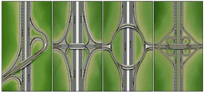
However, crossings between ways and waterways have to be separated vertically in full function anyhow. And they often occur.



Fig. 88 Rivers, canals and brooks	Fig. 89 Superposition races	Fig. 90 Interference with highways	Fig. 91 Interference with highways and railways

When one lays different networks over each other, an interference occurs that defines the number of crossings, and, because of this, the level of investment in civil engineering constructions (Fig. 92).

Fig. 92 Interference between wet and dry networks.

The position of urban areas with respect to orders of magnitude of water and roads dictates their character to a large extent. The elongation (stretching) of networks reduces the need for engineering constructions when their meshes lie in the same direction. If one bundles them together, this also helps to prevent fragmentation. The aim of the ‘dual network strategy’, on the other hand, is to position water, as a ‘green network’, as far way as possible from the roads (in an alternating manner). However, this has the effect of increasing fragmentation.

Fig. 93 shows how different dry and wet networks in different orders cause crossings of different kinds.


	Jong (2001)
Fig. 93 Interference of dry and wet networks in different orders causing crossings of different kinds

Trenches and ditches become drains or underneath roads culverts in the urban area, but main ditches (3m wide), races (10m) and canals (30m) have to be crossed by bridges. From 9 different kinds of crossing Fig. 93 counts 6 types (Fig. 94).

	neigbourhood streets (10m wide)	district roads (20m wide)	city highways (30m wide)
main ditches (10m wide)	2		1
races (30m wide)	3	1
canals (100m wide)	2		1

Fig. 94 Five types of crossings supposed in Fig. 93

Especially when the canal is a belt canal with a higher level then the other waterways many complications arise. Extra space is needed for weirs, dikes and sluices, perhaps even locks and many slopes not useful for building. The slope the city highway gets from crossing the high belt canal could force to make a tunnel instead of a bridge. Anyhow, several expensive bridges will be necessary and some of them will be dropped from the budget, causing traffic dilemmas elsewhere.

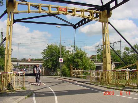
Fig. 95 Neighbourhood street crossing canal and railroad in Utrecht

The slope behind the bridge in Fig. 95 is not steep enough to get a tunnel under the railway high enough for public transport (2.60m is too low).

1.5.3 Bridges

based on pressure	or	draw

arch bridge (boogbrug) approach ramp(aanbrug) thrust (horizontale druk) deck (rijvloer) trussed arch with upper and lower chord (vakwerkboog boog met boven- en onderrrand) abutment (landhoofd)	beam bridge (balk- of liggerbrug) abutment (landhoofd) overpass, underpass (bovenkruising, onderdoorgang) deck (brugdek) continuous beam (doorgaande ligger) pier (pijler) parapet (leuning)	suspension bridge (hangbrug) anchorage block (ankerblok) suspension cable (hangkabel) suspender (hanger) deck (rijvloer) center span (middenoverspanning) tower (toren) side span (zijoverspanning) abutment (landhoofd)

trough arch bridge (boogbrug met laaggelegen rijvloer)	multiple span beam bridge (balk- of liggerbrug met meer overspanningen)	fan cable stayed bridge (waaiertuibrug) cable stay anchorage (tuiverankering)

half-through arch bridge (boogbrug met tussengelegen rijvloer)	viaduct	harp cable stayed bridge (harptuibrug)

deck arch bridge (boogbrug met hooggelegen rijvloer)	cantilever bridge (kraagliggerbrug, cantileverbrug) suspended span (zwevend brugdeel) cantilever span (uitkragende zijoverspanning)	transporter bridge (zweefbrug) trolley (wagen) platform (platform)

fixed two-hinged three-hinged arch (ingeklemde, tweescharnier~, driescharnierboog)	single-leaf bascule bridge (enkele basculebrug) counterweight (contragewicht)	lift bridge (hefbrug) guiding tower (heftoren) lift span (val)

portal bridge (schoorbrug) portal frame (portaal) pier (pijler)	double-leaf bascule bridge (dubbele basculebrug)	floating bridge (pontonbrug) manrope (mantouw) pontoon (ponton)

	Bailey bridge (baileybrug)	swing bridge (draaibrug)
Standaard and Elmar (?)
Fig. 96 Names of Bridges and their components

These types of bridges could be made of steel, concrete or wood. Depending on the material they have a different maximum span (fig. 97).

english name	dutch name	span in m.	notes
multiple span beam bridge	balk- liggerbrug met meer overspanningen	unlimited
viaduct	viaduct	unlimited	old-fashioned
ferry bridge	pontbrug	unlimited
suspension bridge	hangbrug	2000	wind-sensitive
fan cable stayed bridge	waaiertuibrug	1000	wind-sensitive
harp cable stayed bridge	harptuibrug	1000	wind-sensitive
cantilever bridge	kraagliggerbrug, Gerberligger	550
arch bridge	boogbrug	500	steel
trough arch bridge	boogbrug met laaggelegen rijvloer	500	? with draw connection
fixed two-hinged three-hinged arch	ingeklemde, tweeschanier-, driescharnierboog	500	? with draw connection
half-through arch bridge	boogbrug met tussengelegen rijvloer	500	?
deck arch bridge	boogbrug met hooggelegen rijvloer	500	?
beam bridge	balk- of liggerbrug	250	steel truss, framework
arch bridge	boogbrug	200	stiffened bars
floating bridge	pontonbrug	200	military	movable
lift bridge	hefbrug	150	old-fashioned	movable
portal bridge	schoorbrug	150	between supports with tube beam
beam bridge	balk- of liggerbrug	100	steel concrete
beam bridge	balk- of liggerbrug	100	concrete tube beam
transporter bridge	zweefbrug, transbordeur.	100	? old fashioned 1895-1920; 2 in europe left	movable
double-leaf bascule bridge	dubbele basculebrug	100		movable
swing bridge	draaibrug	60	even as aquaduct	movable
arch bridge	boogbrug	50	hout
single-leaf bascule bridge	enkele basculebrug	50		movable
portal bridge	schoorbrug	40	? concrete
beam bridge	plaatliggerbrug	30	or wider with large construction height
beam bridge	balk- of liggerbrug	30
strauszbridge	ophaalbrug	25		movable
beam bridge	balk- of liggerbrug	20	2m wood truss, framework
beam bridge	spoorverkeer staal	15	small construction height
ship bridge	schipbrug	10	? te doesburg	movable
beam bridge	balk- of liggerbrug	10	wood
raft bridge	vlotbrug	10	? floating from under approach ramp	movable
crane bridge	kraanbrug	10	old-fashioned	movable
roll bridge	rolbrug	8	one example 67m	movable
clap bridge	klapbrug	8	without counterweight	movable
	valbrug	5	old-fashioned (castles)	movable
	oorgatbrug	1	for mast only, old-fashioned (hindeloopen)	movable
Bailey bridge	Baileybrug		military
Jong (1996; Jong (1996)
fig. 97 Maximum span of different bridges

The construction height below deck is often limiting factor.

1.5.4 Harbours P.M.

1.5.5 References to Networks and crossings

Hildebrandt, S. and A. Tromba (1989) Architectuur in de natuur, de weg naar de optimale vorm (Maastricht/Brussel) Wetenschappelijke Bibliotheek Natuur en Techniek ISBN 90 70157 81 0.

Jong, H. d. (1996) Handboek Civiele Kunstwerken (losbladig 3 mappen) (Den Haag) TenHagen Stam ISBN 90-70011-18-2.

Jong, H. d. (1996) Video 'Beweegbare stalen bruggen' Handboek Civiele Kunstwerken (Den Haag) tenHagen&Stam bv. Afd. Klantenservice Lezersmarkt.

Jong, T. M. d. (2001) Standaardverkaveling 11.exe.

Standaard, M. and m. Elmar (?) Beeldwoordenboek Zo heet dat Standaard Multimedia; Elmar multimedia.

[a] Mail pattern and calculation to T.M.deJong@bk.tudelft.nl

[b] Perhaps because this restriction combined with mirroring vertically and horizontally has used all possibilities of external connection by two axes (above and below) counting half. So, vertically opening up the whole area makes more vertical sections necessary.

[c] This figure is taken from: Stefan Hildebrandt and Anthony Tromba, Architectuur in de natuur, de weg naar de optimale vorm (Mathematics and optimal form), Wetenschappelijke Bibliotheek Natuur en Techniek, Maastricht/Brussel, 1989, ISBN 90 70157 81 0.

The only network that could compete with this, which has lines running from a rectangular lattice, is a triangular lattice, but it is immediately clear that it is inferior because of its unfavourable perifery:area ratio. For instance, the parallelogram in the thought experiment that became ever more skew matches an angle of 60° in an equilateral triangular lattice. Apart from the disadvantage caused by deviating from the right angle, an extra connecting line is needed to cut the parallelogram into two equilateral triangles.